Excel Choose Function

The CHOOSE Function in Excel returns a value from the given data range (array) when the position (index) is specified by the user. This lookup and reference function of excel is most commonly used to create scenarios in financial models.

• The CHOOSE function returns a value from the list based on a position specified by the user.
• The “index_num” and “value 1” can take any numeric value from 1 to 254.
• The “index_num” and “value 1” are mandatory arguments and can be in the form of a cell reference or formula.
• The “index_num” is truncated to the lowest integer if it is entered as a fraction.
• The CHOOSE function can be combined with functions like the sum, average, RANDBETWEEN, VLOOKUP, and so on, depending on the requirement.

The syntax of the CHOOSE function is stated as follows:

The CHOOSE function accepts the following arguments:

#1 - Index_num: This is the position of the value to choose from. It is a number between 1 and 254. It can also be a cell reference or a function giving a numerical value. It can be in any of the following forms:

• 5
• B2
• “=RANDBETWEEN(2,8)”

Note: If “index_num” is entered as a fraction, it is truncated to the lowest integer at the time of use.

#2 - Value1, , : This is the data list from which a value is to be returned. It can be a set of numbers, cell references, cell references as arrays, text, formulas, or functions. It can be in any of the following forms:

• 1, 2, 3, 4, 5
• Sunday, Monday, Tuesday
• A5, A7, A9
• A2:A7, B2:B7, C2:C7, D2:D7

The “index_num” and “value1” are mandatory arguments. The rest of the arguments are optional.

Let us consider the following examples.

Example #1

We have 6 data points, namely–2, 3, 10, 24, 8, and 11. We want to choose the 4^th element.

We apply the formula “=CHOOSE(4,2,3,10,24,8,11)” or “=CHOOSE(4,A3,A4,A5,A6,A7,A8).”

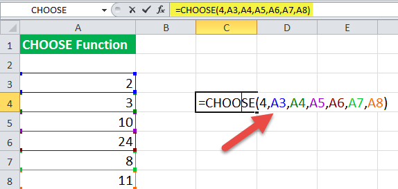
It returns the output 24. If A4 is selected as the index value, it returns 10. This is because A4 corresponds to 3. The third value in the dataset is A5, i.e., 10.

Example #2

We have three columns containing a list of colors, flowers, and numbers. We want to choose a value from the array of values. We want to choose the third value.

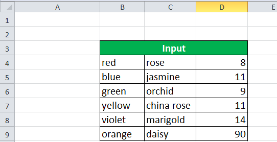
We apply the following CHOOSE formula in Excel.

“=CHOOSE(3,B4:B9,C4:C9,D4:D9)”

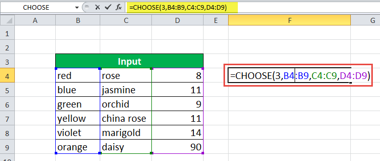
The third value is a list of values “D4:D9,” which is greater than or equal to the input values of column D (8,11,9,11,14,90). So, the output of the formula is the same as the list of values of “D4:D9.”

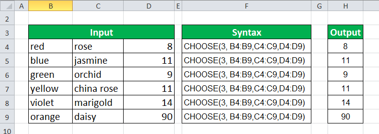
In a single cell, the formula returns only a single value as an output from the list. This selection is not random and depends on the position of the cell in which the answer is required.

In cell F4, the formula “=CHOOSE(3, B4:B9,C4:C9,D4:D9)” gives the output 8, which corresponds to the value in cell D4.

Similarly, in cell F5, the same input gives 11, which corresponds to the value in cell D5.

Example #3

Let us add one more column to our input of the previous example. We apply the following formula to choose the fourth value.

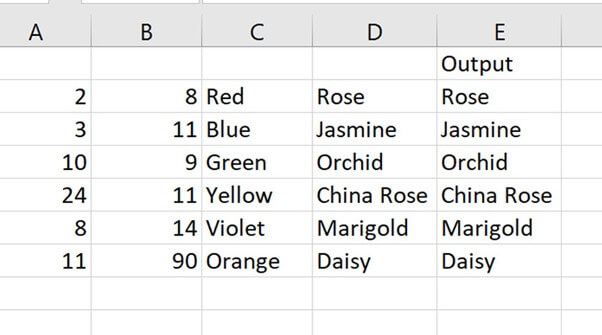
“=CHOOSE(4,A3:A8,B3:B8,C3:C8,D3:D8)”

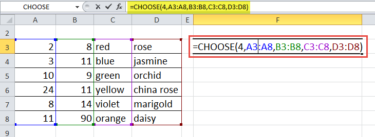
The output is shown in the succeeding image.

Example #4

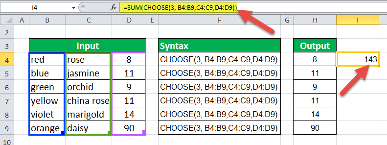
The CHOOSE function can be combined with other functions like the sum, average, mean, etc. Working on the data given in the previous example, we want a sum of “D4:D9.”

We apply the formula “=SUM(CHOOSE(3, B4:B9,C4:C9,D4:D9)).” It gives the sum of the third set of values corresponding to “D4:D9.”

The formula returns the output 143, as shown in the succeeding image.

At times, a random grouping of data is required, like in clinical studies, machine learning, and so on. The CHOOSE function can be used to group data randomly. The following example explains how to group data into different classes randomly.

Example #5

We have a list of 20 subject IDs. We want to group this data into classes–A, B, C, and D.

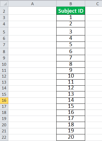
We apply the following formula for selecting the groups A, B, C, and D randomly. “=CHOOSE(RANDBETWEEN(1,4),"A","B","C",”D”).”

The function “=RANDBETWEEN(1,4)” selects a random value between 1 to 4. This function is used here as an index value. So, the index value will be randomized from 1 to 4. This means if the index value is 1, it returns A. If the index value is 2, it returns B, and so on.

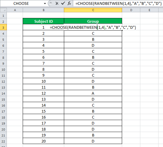
In this way, the data can be classified into any number of classes with the help of the RANDBETWEEN function of Excel.

The CHOOSE function can be used to select a day or month from the given data. The following example explains how to extract and return the month from a date.

Example #6

We have a list of dates in column A. The input values in “A3:A14” are shown in the succeeding image. We want to extract the month for the second date value (A4).

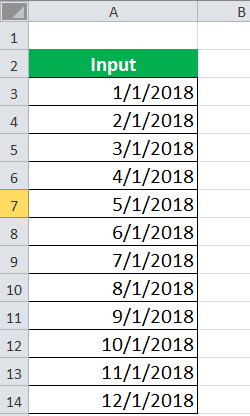
We apply the following formula.

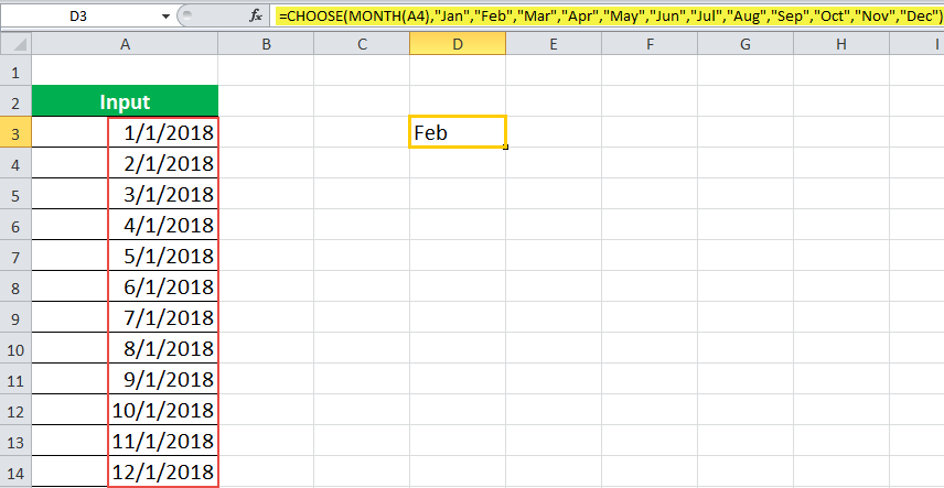
“=CHOOSE(MONTH(A4),"Jan","Feb","Mar","Apr","May","Jun","Jul","Aug","Sep","Oct","Nov","Dec")”

The formula returns “Feb,” as shown in the succeeding image.

The CHOOSE function can be linked with the VLOOKUP function to obtain the desired value.

Example #7

We have a list of student IDs (B6:B12), student names (C6:C12), and marks (D6:D12) as shown in the following image.

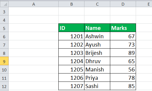
We apply the following formula to find the student's name with the help of the corresponding ID.

“=VLOOKUP(ID,CHOOSE({1,2},B6:B12,C6:C12),2,0)”

Say we want the name corresponding to the ID in cell F6. So, we replace this ID with the cell reference, as shown in the following image.

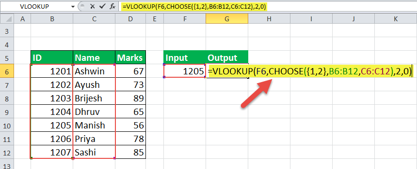
The formula returns the output “Manish.”

Similarly, the marks of a student can be retrieved with the help of the ID or the name. For this, we replace “C6:C12” with “D6:D12.” This returns the output 56.

Example #8

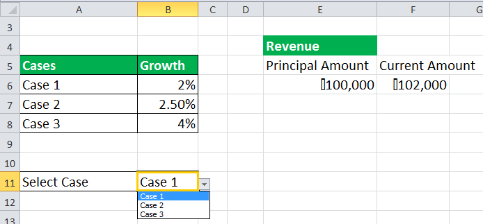
We have three cases with different growth percentages. The principal amount is $100,000. The current amount is “principal amount+(principal amount*growth).” We want the current amount for case 1.

We apply the following formula in Excel.

“=E6+(E6*VLOOKUP(B11,CHOOSE({1,2},A6:A8,B6:B8),2,0))”

This formula is a slight extension of the formula used in Example #7.

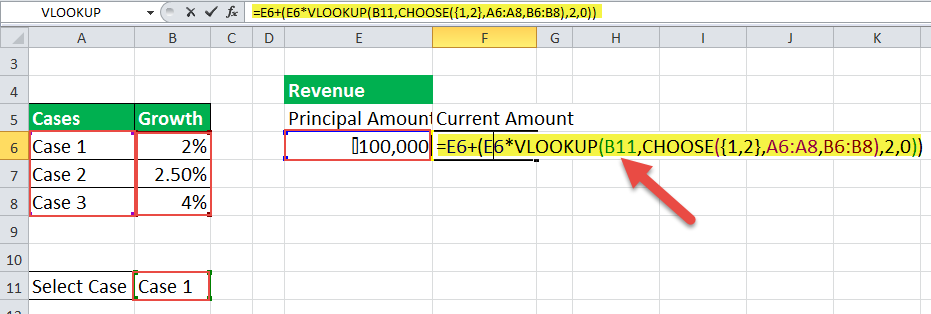
The formula returns the amount of $102,000 for case 1.

1. It returns “#VALUE! error” if:

• the “index_num” argument is greater than the number of values to choose from
• the “index_num” argument does not correspond to a numeric value

2. It returns “#NAME? error” if:

• the value arguments are supplied as text arguments without quotes
• valid cell references are not provided as arguments

This has been a guide to CHOOSE Function in Excel. Here we discuss the CHOOSE Excel Formula and how to use it along with practical examples and downloadable Excel templates. You can have a look at other articles on Excel functions -

• Excel Convert Function
• Excel Mathematical Function
• Max Formula in Excel
• Find Errors in Excel