Table Of Contents
CHAR In Excel
CHAR function in Excel is a function that returns the character specified by the code number (also called the ASCII code) from the character set for your computer. CHAR is categorized as a string/text function. It takes an ASCII value as an input number and gives the character associated with that ASCII value as an output.
ASCII stands for American Standard Code For Information Interchange, a character encoding standard for digital communications. Each character that we can type has a unique integer number associated with it, may it be a character set, digits, punctuation marks, special characters, or control characters. For example, the ASCII value for is 032. In addition, ASCII values ranging from 097-122 are reserved for the alphabets a-z in lower case.
The CHAR function takes the number as input, the ASCII value, and returns the associated character in Excel. So, for example, when we pass 32 as an input, we get a space value as an output.
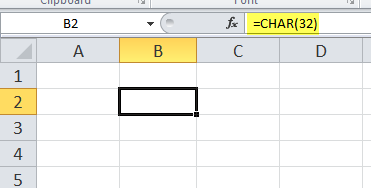
If we copy and PasteSpecial the value of cell B2 to another cell, we will find an as a starting character.
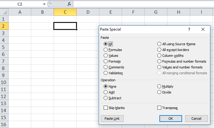
We pasted the value using the “Paste Special” functionality in cell C2, and we have an as a character as an output.
CHAR Formula in Excel
Below is the CHAR formula in Excel.

This CHAR takes a single value as a number where the number is between 1-255.
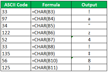
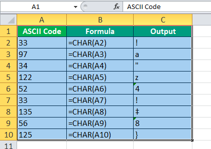
Note: The character code may vary depending on the operating system, so the output may vary on a different operating system for the same input. The WINDOWS operating system uses the ANSI character set, while the MAC OS uses the Macintosh character set.
The CHAR formula has many uses. For example, we can use it to replace unwanted characters. We can further use it while writing an Excel application or a Macro when dealing with strings and characters.
How to Use CHAR in Excel
The Excel CHAR function is straightforward and easy to use. Let us understand the working of the (CHAR) CHARACTER Function in Excel with some examples.
CHAR in Excel Example #1
We have a list of "Characters" in column A with their respective ASCII values, but a few of the "ASCII Values" are incorrect. Therefore, the user needs to find whether the "ASCII Value" is correct and color the wrong "ASCII Value" using conditional formatting.
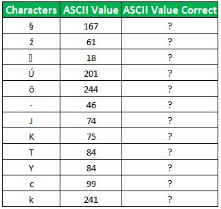
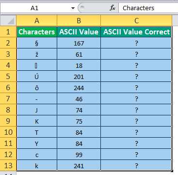
To find whether the "ASCII Value" is correct, we will use the IF condition with the CHAR function in Excel. The formula that we will be using will be
IF CHAR (ASCII Value of given character) matches or equals the given "ASCII Value," then print "Correct"; else, print "Incorrect."
In Syntax, using the reference values, the CHAR formula in Excel will be:
=IF(CHAR(B2)=A2,"Correct","Incorrect")
Applying the above CHAR Formula in the other cells, we have,
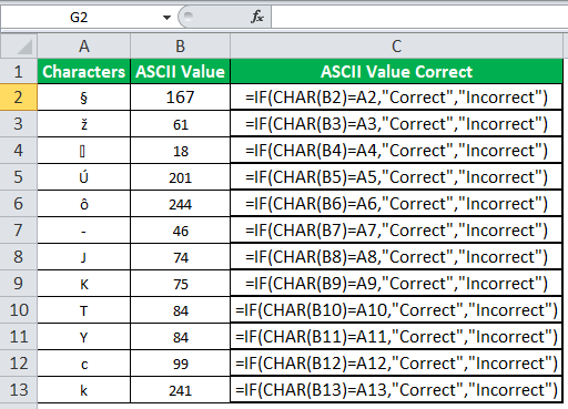
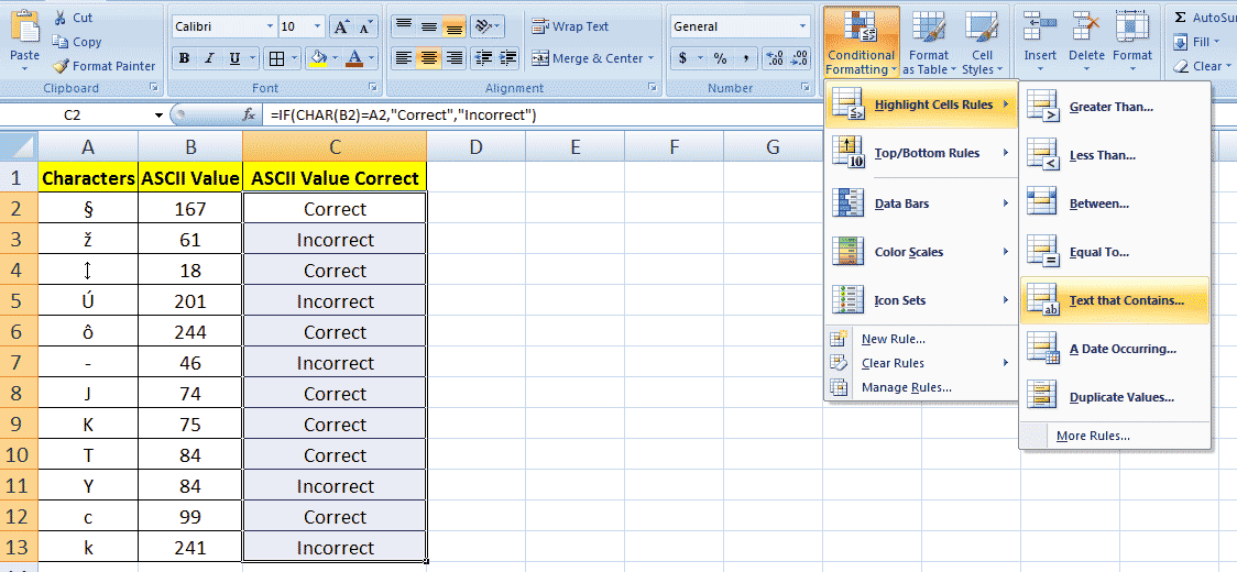
For conditional formatting, select the range we want to apply the condition. Here, the range is C2:C13. Go to Home-> Conditional Formatting -> Highlight Cells Rules ->Text that Contains.
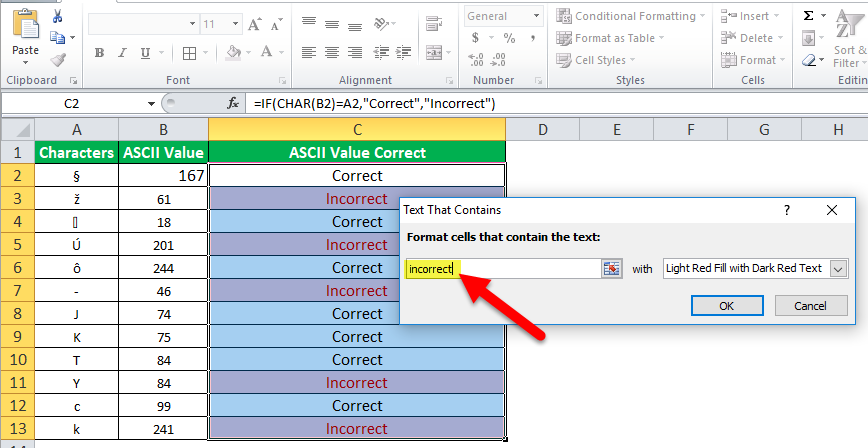
Then, type in the "Text that Contains" to get the cell formatted with the color. Finally, you may specify and enter "OK."
Output:
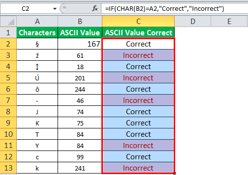
CHAR in Excel Example #2
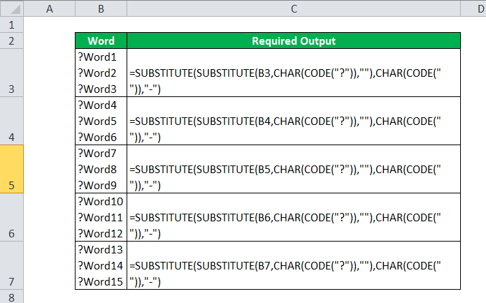
A user downloaded a set of data from the web, and the data downloaded in Excel was in the format given below.
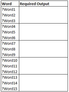
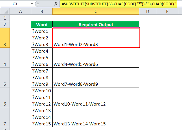
But the user wants the data in a format like Word1-Word2-Word3 and similarly for the data in other cells.
So, we need first to replace or substitute the unwanted characters. Then, we will replace the line breaks to get the desired output.
To replace the unwanted characters, we need to know the ASCII code, so to get the ASCII code, we can use the function named CODE that returns the ASCII value of a character.
The values returned by the Code function can be used as input for the (Char) CHARACTER function in Excel. Further, we will use the SUBSTITUTE function in Excel to replace the unwanted character.
So the CHAR Formula will be:
=SUBSTITUTE(SUBSTITUTE(A2,CHAR(CODE("?")),""),CHAR(CODE("")),"-")
First, we calculated the ASCII code for the '?', 63, and for the 'line break,' the ASCII code is 10. Then, we calculated both values using the CODE function and replaced them with the required output.
Applying the CHAR formula to other cells, we have,
Output:
CHAR in Excel Example #3
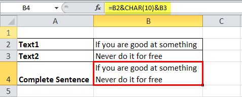
We have two strings in cells B2 and B3, and we want to concatenate both strings with a line break in cell B4.
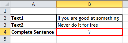
We will use the CHAR in Excel to insert a line break. We know the ASCII code for a line break is 10, so the CHAR formula will be
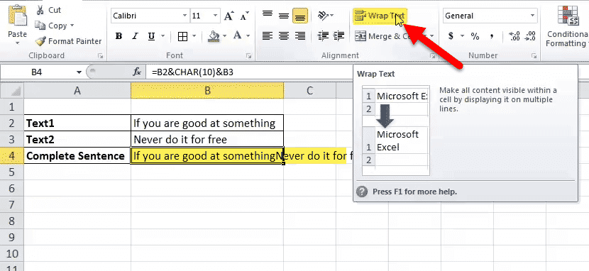
=B2&CHAR(10)&B3
After applying the CHAR formula, we get

Now, to make the content of the B4 more readable and show the line break, we will " wrap text" the content of B4.
Output:
Things to Remember About CHAR Function in Excel
- The (CHAR) CHARACTER function in Excel was introduced in Excel 2000 and later versions of Excel.
- It recognizes the input number between 1-255
- The example shows that we can use it to reverse Excel's (CHAR) CHARACTER function.
- We get #VALUE! Error when we do not supply the number as an input for the (CHAR) CHARACTER function in Excel, and the number is less than 2 or greater than 254.

