CELL Excel Function

What Is CELL Function In Excel?

The CELL function in Excel is an inbuilt Information function. It accepts a cell reference and returns the specified cell’s cited information type, such as its location, content, or format.

Users can use the CELL function when they must analyze massive datasets for errors and the various facets of the information included in them.

For example, the following dataset contains one value in cell A2.

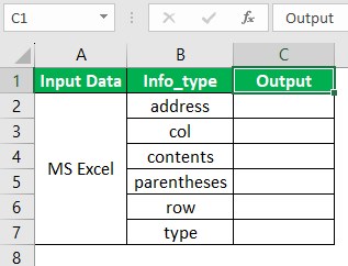
Column B lists the information types we aim to gather about the value given in the source dataset and display them as output in column C.

Then, considering the CELL function definition cited before, we can apply the CELL() in each target cell and obtain the required information.

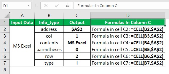
We must find the address of the given source data to display the output as a cell reference in the target cell C2. So, using CELL function in Excel cell C2, with the references to cells containing the required information type and the source data value as inputs, will fetch us the required output. Thus, the cell C2 CELL functionreturns the absolute reference to the cell containing the source data value as the required address, $A$2.

Likewise, cell C3 CELL() returns the source data value column number 1, and in cell C4, the function returns the source data content, MS Excel.

Next, the cell C5 CELL() checks if the cell containing the source data value is formatted with parentheses for all values. And since it is not so, the function returns 0.

On the other hand, the CELL() in cells C6 and C7 determine the source data value row number and data type. Since the source data value is in the second row in the sheet and the data type is text, the function in the corresponding target cells returns 2 and I as the output.

• The CELL function accepts the information type we aim to obtain about a cell and the reference to the specific cell to return the required information pertaining to the cited cell.
• Users can utilize the CELL Excel function to analyze the data in a cell or range for aspects such as data locations, errors, contents, formats, data types and colors.
• The CELL Excel function accepts one mandatory argument value, info_type, and an optional argument value, reference.
• While we can utilize the CELL Excel function as an individual function, using it with other inbuilt functions, such as IF, INDEX and MATCH, yields practical results.

Syntax

The syntax to apply while using CELL function in Excel is the following:

Where,

• info_type: The argument is a text value specifying the information type we want the CELL function to return.
• reference: The cell about which we aim to gather the required information.

While the first argument in the CELL functionis mandatory, the second is optional.

Furthermore, the table below lists the valid text values we can supply as the info_type argument value.

info_type	CELL() Output
"address"	The function returns the reference to the top cell in the reference as a text.
"col"	The function returns the first cell’s column number in the reference.
"color"	The function returns the value of 1 when the first cell in the reference is formatted using color for negative values. Otherwise, the function returns 0.
"contents"	The function returns the value the upper-left cell in the reference contains. Please note that the function does not return the formula but the formula output.
"filename"	The function returns the file name (the full path) of the file containing the reference as a text value. However, it returns an empty text when the sheet containing the reference is not yet saved.
"format"	The function returns the number format of the specified cell as a text. It returns a Hyphen after the text value for the cell formatted in color for negative values. The function output will have the "()" after the text value for the cell formatted with parentheses for positive or all other values.
"parentheses"	The function returns the value 1 when the specified cell is formatted, which includes parentheses for positive or all values. Otherwise, the function returns 0.
"prefix"	The function returns the corresponding text value of the “label prefix” of the cited cell. It returns “'” when the cell has left-aligned text, “"” when the cell has right-aligned text, “^” when the cell contains centered text, “\” when the cell has a fill-aligned text, and empty text when the cell has anything else.
"protect"	The function returns the value 0 for an unlocked cell. Otherwise, the function output is 1, indicating a locked cell.
"row"	The function returns the first cell’s row number in the reference.
"type"	The function returns the data type in the cited cell as a text value.
"width"	The function output is an array with two elements. The first element is the cited cell’s column width, rounded off to an integer. Every column width unit equals one character width in the default font size. The second element is a Boolean value. While the value is TRUE when the column width is the default value, the value is FALSE if the user specifies the width explicitly.

Ensure that when supplying the info_type argument value directly, the value must be in double quotes. Otherwise, the value can be a reference to the cell containing the info_type argument value.

Also, please note that all the info_type argument values help obtain information regarding the first (or the upper-left) cell in the reference argument. On the other hand, the info_type argument values color, filename, format, parentheses, prefix, protect, and width do not work in Excel Web, Excel Mobile, and Excel Starter. The reason is that they do not support these values.

Further, the tables below show the values the CELL function will return in different scenarios when the info_type argument value is “format” and “type”.

Excel Format	CELL() Return Value
General	"G"
# ?/? or # ??/??	"G"
#,##0	",0"
0	"F0"
0.00	"F2"
#,##0.00	",2"
$#,##0_);($#,##0)	"C0"
$#,##0_);($#,##0)	"C0-"
$#,##0.00_);($#,##0.00)	"C2"
$#,##0.00_);($#,##0.00)	"C2-"
0%	"P0"
0.00%	"P2"
0.00E+00	"S2"
d-mmm-yy or dd-mmm-yy	"D1"
d-mmm or dd-mmm	"D2"
mmm-yy	"D3"
m/d/yy or m/d/yy h:mm or mm/dd/yy	"D4"
mm/dd	"D5"
h:mm:ss AM/PM	"D6"
h:mm AM/PM	"D7"
h:mm:ss	"D8"
h:mm	"D9"

Data Type	CELL() Return Value
Blank	"b"
Text	"l"
Others	"v"

Please note that if the info_type argument value in the CELL() is "format". Next, when we apply a different format to the specific cell in question, we must re-evaluate the sheet (F9) to update the CELL() output.

Furthermore, the reference argument value is usually a cell reference. However, if the supplied reference argument value is a range, the CELL() output is the information about the upper-left cell of the range.

On the other hand, if we omit the reference argument value, the information based on the info_type argument is returned for the last modified cell.

The Excel CELL function examples explained later in the article will help understand the CELL() argument values settings better.

However, the suggestion is to avoid ignoring the second argument value. Otherwise, the CELL() output can be affected due to the following reasons:

• In the case of automatic calculation mode, when a user modifies a cell, the calculation triggers before or after the selection has commenced. It depends on the platform we use for Excel.
• When we Co-Author with another user who edits the worksheet, the CELL() will report our active cell rather than the editor’s.
• In the case of recalculation, for instance, pressing F9 will make the function return a new output even though we do not edit any cell.

Please note that the abovementioned syntax and the CELL() facets are applicable for the CELL function Google Sheets as well.

How To Use CELL Excel Function?

We can utilize the CELL function in two ways:

1. Access the function from the Excel ribbon.
2. Enter the function into the worksheet manually.

Method #1 – Access The Function From The Excel Ribbon

Choose a target cell for output - the Formulas tab - the More Functions down arrow - The Information function group right arrow - CELL.

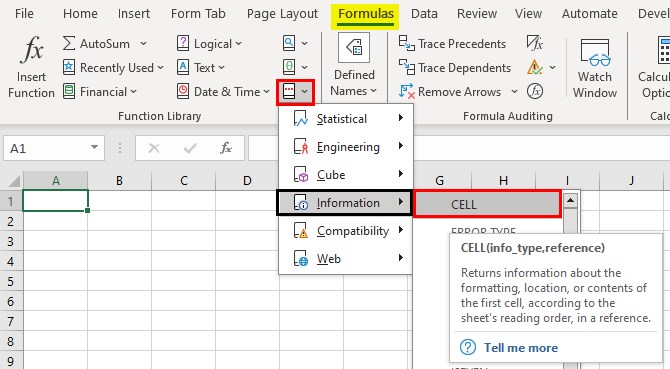
The Function Arguments window will appear. Enter the argument in the Info_type and Reference fields based on the CELL function definition and syntax.

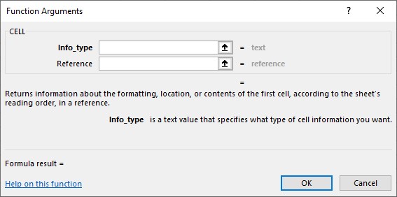
Finally, clicking OK in the Function Arguments window will show the CELL() output in the target cell.

Method #2 – Enter The Function Into The Worksheet Manually

1. Choose a target cell to show the output.
2. Type =CELL( in the cell.
3. Enter the arguments as values or cell references and close the brackets.
4. Press Enter to view the CELL() output.

Please note that the above methods will work for CELL function Google Sheets as well.

Examples

Check out the following Excel CELL function examples to use it effectively.

Example #1 - Finding A Certain Value

The first dataset lists sales representatives and the sales they generated in January.

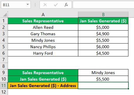
The second dataset shows a sales representative and the sales they generated in cells B9:B10. The aim is to find the sales-generated value of the sales representative specified in the second dataset in the first dataset as a cell address. Assume the target cell is B11.

Then, here is how to use the CELL function with the Excel INDEX function and MATCH function in the target cell to obtain the desired output.

Step 1: Choose cell B11, enter the CELL() containing the INDEX and MATCH functions, and press Enter.

=CELL("address",INDEX(B2:B6,MATCH(B9,A2:A6,0)))

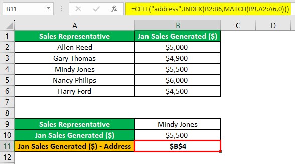
First, the MATCH() finds the relative position of the specified sales figure of $5,500 in the cited array A2:A6. Since the given value is in the third position in the array, the MATCH() returns the value 3.

Next, the INDEX() returns the reference or the value at the intersection of the specified column B2:B6 and the row, which the MATCH() returned, 3. Thus, the INDEX() returns the absolute reference of the cell at the intersection, $B$4.

Finally, since we must find a value and display the output as a cell address, we supply the info_type argument value in the CELL() as “address”. Thus, the CELL() returns the address of the specified cell reference, $B$4, as the required output.

Example #2

The following dataset shows the results of five experiments.

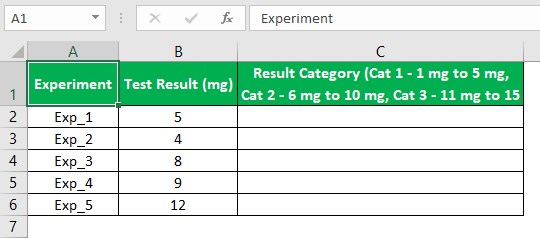
The aim is to determine the category of each experiment result based on the categories specified in cell C1. Assume the target cells are in column C.

Then, we can use the CELL function in Excel IF function in each target cell to obtain the required outcome.

Step 1: Choose cell C2, enter the IF() containing the CELL(), and press Enter.

=IF(CELL("contents",B2)>10,"Cat 3",IF(CELL("contents",B2)>5,"Cat 2","Cat 1"))

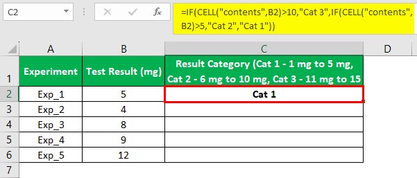
Step 2: Using the Excel fill handle, implement the formula in the remaining target cells.

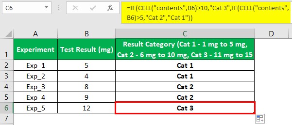
Let us check the cell C6 formula to understand its logic.

The CELL function in the outer IF() condition returns the cell B6 content, 12. Next, the formula checks if the CELL() output, 12, is greater than 10. Since the IF condition is true, the IF() returns the TRUE value, Cat 3.

Example #3

The following image shows a source dataset containing a list of employees and their designations and company email IDs.

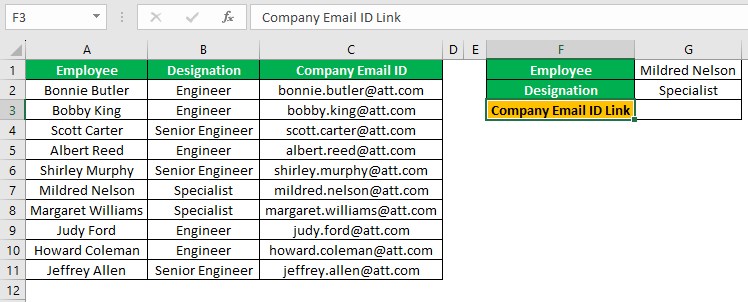
The second dataset shows a specific employee and their designation.

The aim is to create a hyperlink to the specified employee's email ID to jump to the exact match in the source dataset by clicking the link. Assume the target cell is G3.

Then, we can use the CELL function with the Excel HYPERLINK function, INDEX, and MATCH functions in the target cell to get the required hyperlink.

Step 1: Choose cell G3, enter the following formula, and press Enter.

=HYPERLINK("#"&CELL("address", INDEX(C2:C11, MATCH(G1,A2:A11,0))), "Click Here")

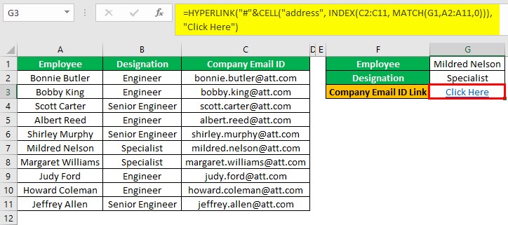
Now, we can click the link in cell G3 to directly jump to the cell containing the specified employee’s email ID in the source dataset.

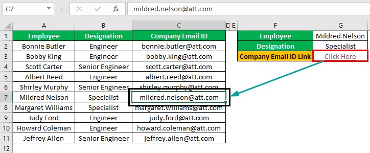
First, the MATCH() determines the relative position of the specified employee name,  Mildred Nelson, in the cited array A2:A11. Since the given value is in the sixth position in the array, the MATCH() returns the value 6.

Next, the INDEX() returns the reference or the value at the intersection of the specified column C2:C11 and the row, which the MATCH() returned, 6. Thus, the INDEX() returns the absolute reference of the cell at the intersection, $C$7.

Next, since we must determine the output as a cell address, we supply the info_type argument value in the CELL() as “address”. Thus, the CELL() returns the address of the specified cell reference, $C$7, as the required output.

After that, the formula concatenates the ‘#’ symbol and the absolute cell reference we obtained as the CELL() output. The result becomes the HYPERLINK()’s first argument, link_location, with the phrase “Click Here” being the second argument value, friendly_name.

Thus, the HYPERLINK() creates the link to jump to the required value directly, which is the specific employee’s email ID in the source dataset.

Important Things To Note

• Ensure to supply an info_type argument value that the CELL function recognizes. Otherwise, the function return value will be the #VALUE! error in Excel.
• Ensure the info_type argument value is in double quotes when supplying the value directly to the CELL Excel function. Otherwise, the function output will be the error value #NAME?.
• The suggestion is to supply the second argument, reference, to the CELL Excel function, though the argument is optional. Otherwise, we may face issues when using the automatic calculation mode, co-authoring the worksheet with another user, and during recalculation.

Frequently Asked Question (FAQs)

Download Template

This article must be helpful to understand the CELL Function, with its formula and examples. You can download the template here to use it instantly.

Recommended Articles

This has been a guide to What Is CELL Excel Function. Here we learn the CELL function syntax and how to use it in Excel with examples and points to remember. You can learn more from the following articles –

• Go To Special Excel
• New Line in an Excel Cell
• Combine Cells In Excel