Excel CEILING Function

Last Updated :

21 Aug, 2024

Blog Author :

Edited by :

Ashish Kumar Srivastav

Reviewed by :

Dheeraj Vaidya, CFA, FRM

Table Of Contents

arrow

CEILING Function in Excel

The Excel CEILING function is very similar to the floor function in Excel. Still, the result is just the opposite of the floor function. The floor function gives us the result of the less significance and CEILING formula provides us with the result of higher significance. 

So, for example, if we have the number 10 and significance as 3 then 12 will be the result.

Syntax

CEIling Formula

Compulsory Parameter:

  • number: It is the value that you want to round off.
  • significance: It is the multiple that we want to round up.

How to Use the CEILING Function in Excel?

Example #1

Let us take a set of positive integers as number arguments and positive numbers as significance, then apply the CEILING Excel function below. It will show the output in the result.

Excel CEILING function Example 1

Example #2

In this example, we take a set of negative integers as number arguments and positive numbers as significance, then apply the CEILING Excel formula as shown in the table below. The output will be shown in the result as follows:

Excel CEILING function Example 2

Example #3 

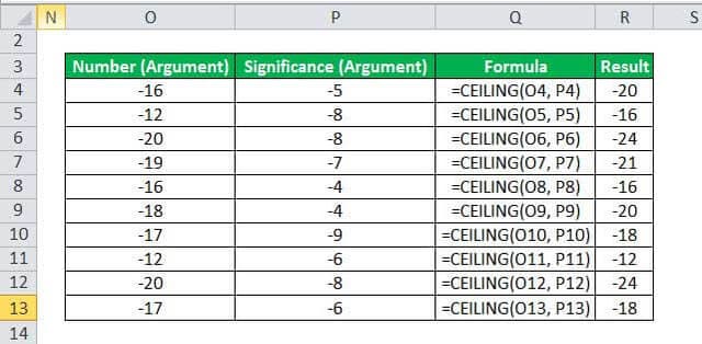
In this example, we take a set of negative integers as number arguments and negative numbers as significance, then apply the CEILING Excel formula to it.

Excel CEILING function Example 3

Example #4

We can use the excel CEILING formula to highlight the rows in the group of given data, as shown in the below table. We will use the CEILING in Excel with ROW and ISEVEN functions.

Suppose we are given the data below:

Excel CEILING function Example 4

And, If we wish to highlight the rows in the given groups of 3, we can use the Excel formula: =ISEVEN(CEILING(ROW()-19,3)/3) in conditional formatting, and the output will be as follows:

CEILING Example 4-1

Things to Remember

  • #NUM! error:
    • It may occur in MS Excel 2007 or earlier versions. For example, if we provide the significance argument with a different arithmetic sign from the given number argument, get #NUM! Error.
    • It occurs if you are using MS Excel 2010/2013, then CEILING functions through #NUM! Error if the given number is positive and the supplied significance is negative.
  • #DIV/0! Error occurs when the significance parameter is zero.
  • #VALUE! Error occurs when any of the parameters is non-numeric.
  • Excel CEILING function is the same as MROUND, but it always rounds up away from zero.
This article has been a guide to the CEILING function in Excel. Here we discuss the CEILING formula in Excel and how to use the CEILING function and Excel example, and downloadable Excel templates. You may also look at these useful functions in Excel: -