Calculate Percentage in Excel Formula

Last Updated :

Blog Author :

Edited by :

Reviewed by :

Table Of Contents

How to Calculate Percentage Using Excel Formulas?

The percentage is calculated as the proportion per hundred. In other words, the numerator is divided by the denominator and the result is multiplied by 100. The percentage formula in Excel is = Numerator/Denominator (used without multiplication by 100). To convert the output to a percentage, either press "Ctrl+Shift+%" or click "%" on the Home tab's "number" group.

Let us consider a simple example.

On a 15-day vacation, Mr. A spent 10 days in his hometown and 5 days in the USA. What percentage of days did he spend in the USA?

The calculations are given as follows:

Percentage formula=Portion days/Total days*100
Percentage of days spent in the USA=5/15*100=33.33%
Percentage of days spent in hometown=10/15*100=66.66%

Hence, Mr. A spent approximately 33% of his vacation period in the USA.

How to Calculate Percentage Using Excel Formulas?

Let us go through the following examples to understand the concept of percentage in Excel.

Example #1

The following table shows the subject-wise marks of 6 students in a school. Since the results pertain to the annual examinations, the maximum marks of every subject are 100.

We have to calculate the percentage of marks for all students.

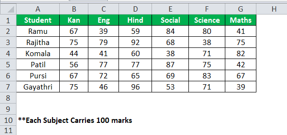
The steps to calculate percentages in Excel are listed as follows:

Calculate the total marks obtained by the students. For this, the marks of every subject are added.
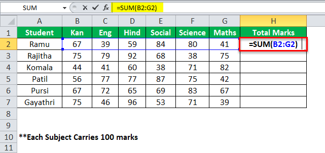
Drag the formula of cell H2 to get the total marks obtained by all students. The output is shown in the following image.
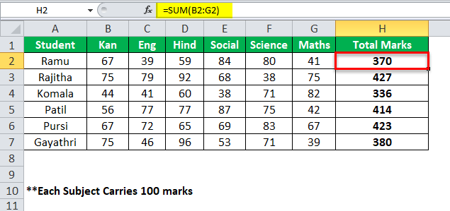
Divide the total marks by 600. The values of the “total marks” column become the numerator. Since the number of subjects is 6, the maximum marks are 600 (100*6=600). This becomes the denominator.
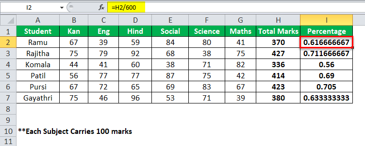
Apply the following formula.

Percentage=Marks scored/Total marks*100.

For percentage values (shown in the succeeding image), change the cell formatting. Select column I and press “Ctrl+Shift+%.” Alternatively, select “%” in the “number” group of the Home tab.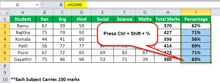

Example #2

The following table consists of students who undertake internship in an organization. Their task is to sell products based on pre-defined targets.

We want to determine the efficiency level (percentage) of every student.

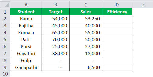
The steps to calculate the efficiency level are listed as follows:

Step 1: Apply the formula “sales/target.”

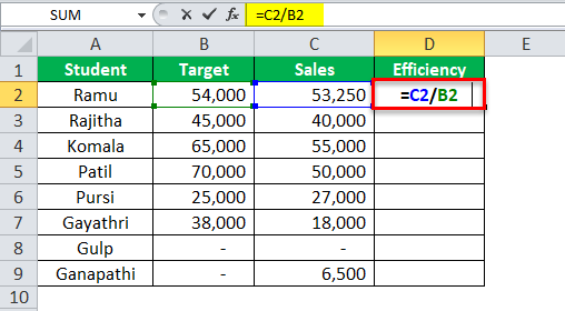
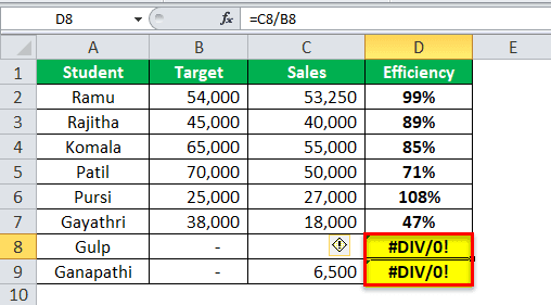
Excel Formula for Percentage example 2-1

Step 2: Format column D to obtain the efficiency levels in percentage. For the last two students (Gulp and Ganapathi), the formula returns “#DIV/0!” error.

Note: If the numerator is zero, the division of the numerator by the denominator returns “#DIV/0!” error.

Excel Formula for Percentage example 2-2

Step 3: To eliminate the error, tweak the existing formula as “=IFERROR(C2/B2,0).” This implies that the IFERROR displays zero if the division of C2 by B2 returns an error.

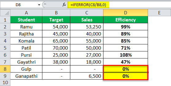
In other words, the “#DIV/0!” error is replaced by zero with the help of the modified formula.

Note: The IFERROR function helps get rid of percentage errors.

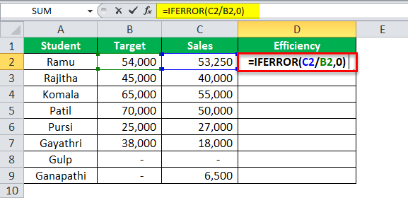
Step 4: The output using the IFERROR function is shown in the following image. The efficiency levels of students Gulp and Ganapathi are zero. This is because of the blank (zero) in column B and/or column C.

Example #3

For 2018, an organization's sales for the months January and February are given in the following table.

We want to calculate the growth or the decline (percentage) in monthly sales.

The steps to calculate the increase (growth) or decrease (decline) percentage are listed as follows:

Step 1: Apply the formula “=(C2-B2)/B2.”

The sales in February (57500) are more than the sales in January (53250). The difference (growth) between the two sales is divided by the sales of the initial month (January).

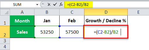
Step 2: Format column D to obtain the growth percentage.

Hence, the February sales have increased by 7.98% over January sales.

Note: While calculating the growth or decline percentage, if the numerator or the denominator is less than zero, the output is a negative value.

Frequently Asked Questions

1. What is the Excel formula for percentage?

The basic percentage formula is “(part/total)*100”. This formula is used in Excel without the latter part (*100). This is because when the percentage format is selected, the resulting number is automatically changed to percent.

In addition, the decimal points are removed and the output is shown as a rounded percentage. For instance, 26/45 is 0.5777. By applying the percentage format, this decimal number becomes 58%.

To convert the output to percentage, either press “Ctrl+Shift+%” or select “%” in the “number” group of the Home tab.

2. What is the Excel formula for calculating the percentage change?

The formula for calculating the percentage change is stated as follows:

“(New value-Initial value)/Initial value”

This formula helps calculate the percentage increase or decrease between two values. A positive percentage implies an increase, while a negative percentage shows a decrease.

Note: To get the final answer (percentage change), the percentage format is applied to the output of the formula.

3. What is the Excel formula for calculating the percentage of the total?

The formula for calculating the percentage of the total is “(part/total).” For instance, column A lists the monthly expenses from cell A2 to cell A11. The cell A2 contains $2500 as the rent paid. The cell A12 contains the total expenses $98700.

The formula “=A2/$A12” returns 3% after applying the percentage format. This implies that the rent is 3% of the total paid expenses.

Since A2 should change on dragging the formula to the remaining cells, it is entered as a relative reference. On the other hand, the total should remain fixed for all cells, so A12 is entered as an absolute reference.

The percentage is the proportion per hundred.
To calculate the percentage, the numerator is divided by the denominator and the result is multiplied by 100.
For obtaining percentages, the output column is formatted by pressing “Ctrl+Shift+%” or selecting “%” in the Home tab.
The division of the numerator by the denominator returns “#DIV/0!” error if the former is zero.
The percentage errors can be removed with the help of the IFERROR function.
The increase or decrease percentage is calculated by dividing the difference between two numbers with the initial number.