Border In Excel

Last Updated :

Blog Author :

Edited by :

Reviewed by :

Table Of Contents

What Are The Borders In Excel?

Border in Excel is the outline given for the data tables or a specific range of cells. In Excel, borders are used to separate the data in borders from the rest of the text. It is a good way of representing data. In addition, it helps the user to look for specific data easily. These borders are available in the “Home” tab in the fonts section.

What are the Borders in Excel?

Border in Excel helps users to create a presentable and organized dataset that is easy to read and understand.
When we use Borders, we can differentiate between the cell values in the datasets, such as headers or headings of the dataset, details that are added under different headings, any formulas or formula results, etc.
With the help of the “Conditional Formatting” option, we can create a rule to automatically add Border in Excel, and use the “Format Painter” option to copy the border formatting to the moved, cut, or copied cells.

Explanation Of Border In Excel

We can add the border to a single or multiple cells, or a cell range. Borders are of different styles and can be used as per the requirement. It also helps present the data set in an organized format in Excel.

We can use borders for tabular format data or headlines to emphasize a specific set of data or can be used to distinguish different sections as,

We can use it to define or divide the sections of a worksheet.
We can use it to emphasize specific data.
We can also make the data more understandable and presentable.

How To Create/Add Borders In Excel?

We can create and add borders to the specific set of data as follows:

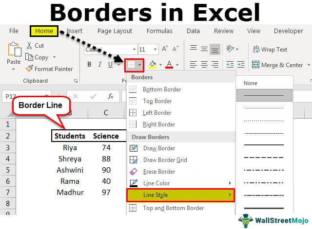
First, choose the cells or the cell range - select the “Home” tab - go to the “Fonts” group - click the “Borders” option drop-down - select the desired options from the list, as shown below.

Examples

We will consider some examples to apply Borders in Excel.

Example #1

We have data of the marks of a student for three subjects of an annual examination. We must add the borders in this data to make it more presentable.

Now, we must select the data we want to add to the borders.
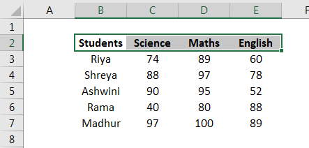
In the font group on the “Home” tab, click the down arrow next to the “Borders” button. You will see the drop-down list of borders, as shown in the figure below.
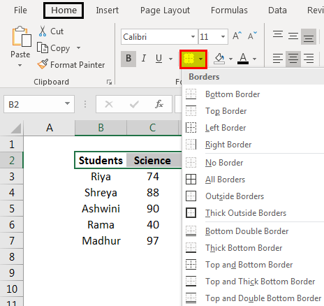
We have different border styles. Therefore, we will select the “OUTSIDE BORDERS” option for our data.
We will get the border shown below, by using “OUTSIDE BORDERS” in the data.

Example #2

We have data of the marks of a student for three subjects of an annual examination. We must add the borders in this data to make it more presentable.

Data of marks of 5 students for three subjects in an annual examination is shown below.

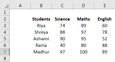
Now, we must select the data we want to add to the borders.

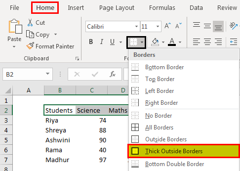
Now, in the “Font” group on the “Home” tab, we need to click the down arrow next to the “Borders” button. As shown in the figure below, we will see the drop-down list of borders.

Now that we have different border styles, we must select the “THICK OUTSIDE BORDERS” option for data.

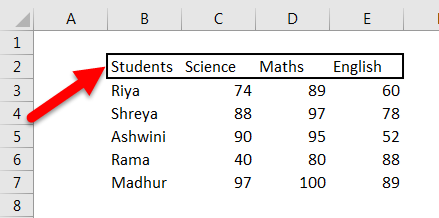
As a result, we get the “THICK OUTSIDE BORDERS” to the data, as shown below.

Example #3

We have data of the marks of a student for three subjects of an annual examination. We must add the borders in this data to make it more presentable.

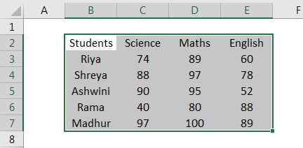
Data of marks of 5 students for three subjects in an annual examination is shown below.

Now, select the data to which you want to add borders.

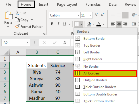
Now, in the “Font” group on the “Home” tab, we will click the down arrow next to the “Borders” button. And we see the drop-down list of borders as shown in the figure below. Then, select the “ALL BORDERS” options for the data.

As a result, we see “ALL BORDERS” in the data, as shown below.

Example #4

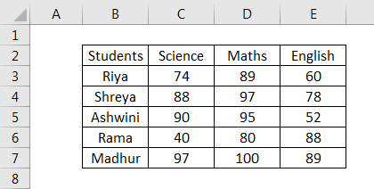
We have data of the marks of a student for three subjects of an annual examination. We must add the borders in this data to make it more presentable.

Data of marks of 5 students for three subjects in an annual examination is shown below.

Now, we must select the data we want to add borders.

Now, in the “Font” group on the “Home” tab. Then, we must click the down arrow next to the “Borders” button. As shown in the figure below, we see the drop-down list of borders. Now, select the “ALL BORDERS” options for our data.

We now find the result using “ALL BORDERS” in the data, as shown below.

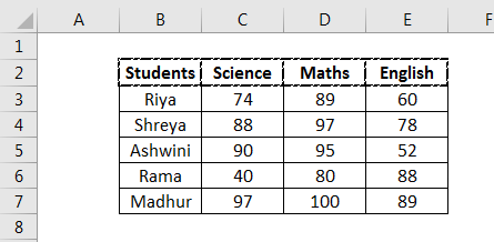
In the figure below, we will now change the border’s thickness as per the requirement. Therefore, select the data that you want to change the border’s thickness for.

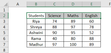
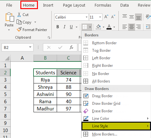
We must go to the border drop-down list and click “LINE STYLE.”

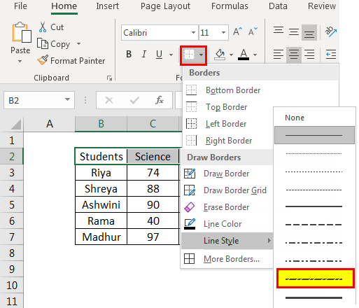
Now, we get a list of line styles and use the style as per the requirements. We will use the second last line style for our data.

We get the result, as shown below.

Important Things To Note

When we apply borders to a dataset, it will stay as it is unless we update the data, like when we copy-paste, or move data, we will lose the border formatting for the particular cell that we moved or cut.
We can select a single cell or a cell range to apply various border options available in the “Borders” icon in the “Font” tab.
When we insert a column or a row within an existing dataset, the borders formatting will get updated automatically. If it doesn’t copy, then we can reapply the borders formatting or use the “Format Painter” option to copy- paste the border format.

Frequently Asked Questions

1. How to remove Border in Excel?

We can remove the Border in Excel in a dataset that already has some borders selected, as follows:
• Choose the dataset for which you want to remove borders.
• Select the “Home” tab - go to the “Fonts” group - click the “Borders” option drop-down - select the “No Border” options from the list, as shown below.

2. How to automatically add a Border in Excel?

We can automatically add Border or Borders in Excel by creating a “New Rule…” in the “Conditional Formatting” option in the “Styles” group of the “Home” tab.

Conditional Formatting - New Rule

3. How to take a Printout with Border in Excel?

The procedure to take a printout with the border formatting is,
• First, select the worksheet that we want to print.
• Then, select the “Page Layout” tab - go to the “Sheet Options” group - check/tick the “Print” option checkbox under the “Gridlines” category, as shown below.

Page Layout - Print

• Finally, click the shortcut keys “Ctrl+P” to take a printout with the border formatting.