Table Of Contents
What Is Binomial Option Pricing Model?
The binomial option pricing model is employed to calculate the value of an option using an iterative binomial framework. It is based on the presumption that the underlying asset's value follows a path of evolution. Hence it either increases or decreases by a fixed percentage during each period.

Investors and traders can analyze their stock options using the tools provided by the model. For example, they can use a binomial tree to project all potential values for the underlying asset when the option expires and, from those values, all possible final values for the option. Then, they can adjust trading strategies and portfolios accordingly.
Table of contents
- The binomial option pricing model helps calculate an option's value. In the model, the value of the underlying asset follows a path of evolution so that it either increases or decreases by a fixed percentage during each period.
- The model works on the key assumption that only two possible results exist for a particular stock.
- It is simpler to use than other models. The option price and the underlying stock price can be compared. Additionally, it enables an investor to examine several periods for an option up until the expiration date.
Binomial Option Pricing Model Explained
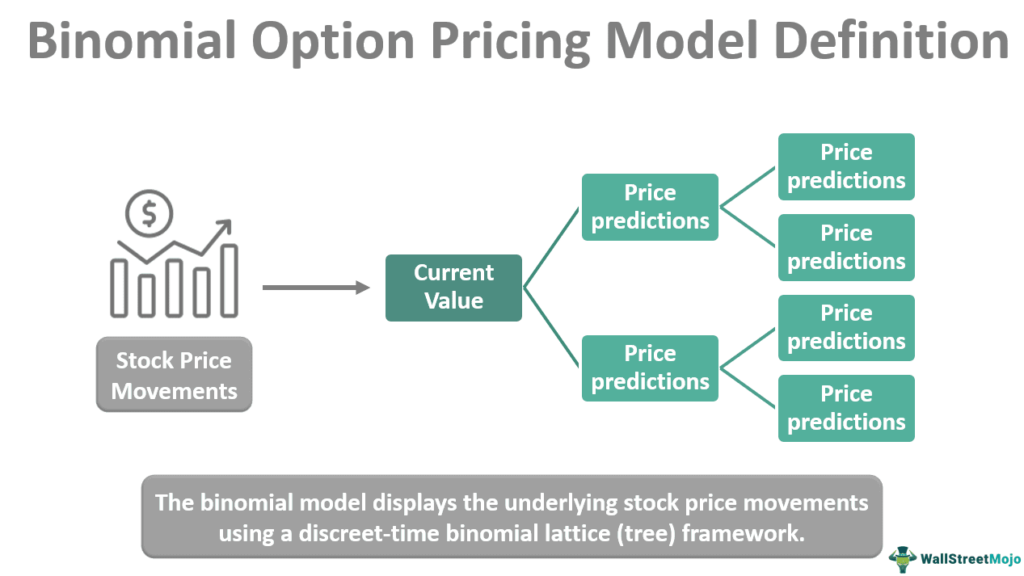
The binomial pricing model was first proposed by mathematicians Cox, Ross, and Rubinstein in 1979. The model provides a simple way to portray stock price movements and the interest rate term structure. The binomial model displays the underlying stock price movements using a discrete-time binomial lattice (tree) framework. One can identify it just by the probability of an upward rise and the size of the moves in the upward and downward phases of the options.
An option is a significant financial derivative that provides the holder with the right to trade a defined quantity of the underlying asset at an agreed amount on the maturity date (for a European option) or at any time on or before the maturity date (for an American option). But they are not obligated to do so. For example, with a call option, the holder can buy, but there is no requirement. With a put option, the holder can sell but have no obligation to sell.
Furthermore, the strike price is a predetermined price, and the expiration date is the date on which the period ends. The option holder exercises the option if they take advantage of it. It is typically the case that an option is out of the money if it is exercised after or on the expiration date. If the option is out of the money, the option holder will not profit financially from exercising the option.
The strike price is the same as the underlying asset when the option is at the money, and typically holders gain when the option is in the money (more than the strike price). These form the basic terms of options trading. In the binomial lattice option pricing model, initial assumptions about the price are made, and the process is optimized in the later stages. As a result, the model generates several accurate estimations before arriving at a final figure.
An investor will be aware of the current stock price, and this price will be the basis for future predictions. Therefore, investors must predict the stock price on the option's expiration date. Hence, two possible option prices are present at the expiration date and a probability value. Therefore, the one-period time model or one-period binomial option pricing model and the multi-period binomial option pricing model or two-step binomial option pricing model are the binomial models one uses to determine option prices.
Assumptions
The binomial lattice option pricing model (also known as the two-state option-pricing model or two-step binomial option pricing model) is a simple approach to calculating possible option prices. The model works on the key assumption that only two possible results exist for a particular stock. The two possible outcomes are a high and a low price. So the possibilities are also an assumption that the prices could go up or down. Therefore, investors need to assume the occurrence of the two stock prices at the end of the provided period. As always, one cannot predict this price with certainty, and it carries risks like all investments.
It also works with the assumption of no arbitrage. i.e., there is no buying while selling at a higher price. No-arbitrage guarantees that the asset's value doesn't change. According to the no-arbitrage supposition, all risk-free investments generate a risk-free rate of return, and no investment possibilities demand zero money and generate positive returns.
The practices ensure that the prices of financial assets, such as options, are fixed to a minimal tolerance from their theoretical values. One-period time model or one-period binomial option pricing model and multi-period binomial option pricing model or two-step binomial option pricing model are the types of binomial models used to determine option prices, and assumptions apply to them too.
Calculation Example
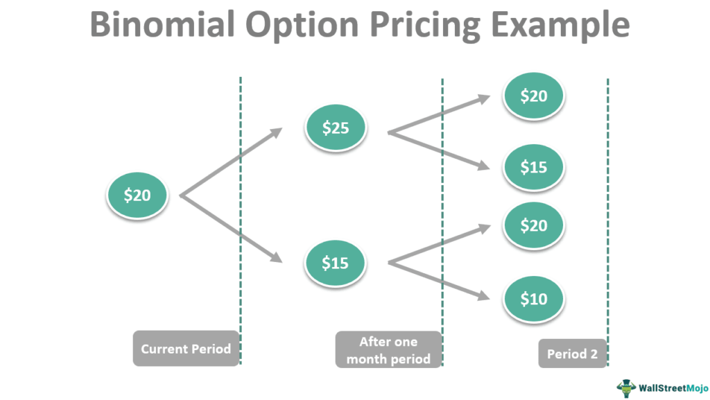
Let's assume the current price of an option is $20, and the investor expects the prices to shift between $25 and $15. This is the current situation. The binomial method enables us to move to the next period, assuming the next course of action should occur within a month. During that period, volatility factors could kick in, and the prices could shift from the two initial predictions.

The first prediction was $25, and the second was $15. From the first initial prediction, i.e., $25, the price could vary between $20 and $15; and from the second initial prediction, i.e., $15, the price could vary between $20 and $10. At each node, one can determine various option values. For example, the first month's option strike price was $20.
If the price had increased to $25, the option would be worth $5, and if the value were decreased to $15, there would be no return. This evolution process gives the investor the freedom to choose the desirable price.
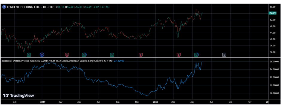
Below is an explanation of the model using a chart taken from TradingView. This model has been used in the chart of Tencent Holding Ltd. It is to be noted that both American and European vanilla options can be priced using this model. In the calculation, first, the time left till expiry is divided into equal parts. However, the model can be presented using two or more than two steps, which consist of those parts. So if there are 60 days left to expiry, the tree can have two steps, each of 30 days.
Each step will end with a node consisting of the price. The price expectation will be based on the price fluctuation of the underlying asset. Thus, after calculating the asset’s price, the option price will be calculated. The calculation will be done backward, within the tree. The steps the trader should follow are, firstly, enter the strike price, dividend yield, and risk-free rate. Secondly, select the type of asset. Thirdly, select the style of option, European or American, along with the type, long call or long put, etc. Lastly, enter the time till expiry and the timeframe of the chart.

Advantages And Disadvantages
Here are the main advantages and disadvantages of the binomial option pricing model:
| Advantages | Disadvantages |
|---|---|
| The model presents a summary of the underlying stock's price over time and provides transparency into the underlying value of the option. | The process of valuing the option is longer. This is because the calculations will take more time than other models if many possibilities are considered. |
| An investor might examine the underlying stock's price at each period, contrast it with the change in the option price, and incorporate different probabilities at each step. | It is not very helpful if the calculation is for many possibilities swiftly (due to the above-mentioned point). |
| This offers a substantial advantage for American-style options compared to alternative pricing methods. In addition, this facilitates checking the options anytime before they expire. | Market forces decide the real values of options contracts, not a complicated formula; hence is a major shortcoming of all pricing models. |
Frequently Asked Questions (FAQs)
In this model, the option expiration time is divided into equal periods, and each period is evaluated by monitoring the up and downward movements of option prices and their probabilities. It is most useful for American-style options, as investors can exercise them anytime.
The binomial option pricing model is important as it is simpler to use than other models. The option price and the underlying stock price can be compared. Additionally, it enables an investor to examine several periods for an option up until the expiration date.
The Black Scholes model works on fixed inputs such as current stock and strike price, the time before expiration, rates without risks, volatility, and dividend yield. Binomial models, in contrast, include expiration time at intervals. The model uses volatility and expiration to forecast two potential moves for the stock price (up and down) at intervals.
Recommended Articles
This has been a guide to what is Binomial Option Pricing Model. Here, we explain its assumptions, calculation, example, advantages, and disadvantages. You can learn more about financing from the following articles –
