Beta Distribution

Published on :

21 Aug, 2024

Blog Author :

Edited by :

Reviewed by :

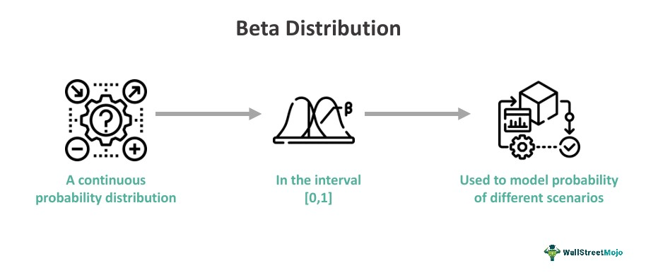
The beta distribution is a continuous probability distribution that is defined on the interval . It allows for capturing different shapes of failure rate curves and provides a valuable framework for assessing the reliability and lifetime distribution of products or systems.

In areas such as market share estimation, quality control, and marketing conversion rate analysis, practitioners commonly apply it as a flexible framework for representing uncertainty in quantities. Hence, this method features two shape parameters, often denoted as α (alpha) and β (beta), both being positive real numbers.

What Is Beta Distribution?

The beta distribution is a continuous probability distribution in the range of commonly used to model the distribution of random variables that represent proportions or probabilities.
It is a tool for decision-makers to assess the potential range of outcomes and make informed choices. Therefore, it is based on the estimated probabilities associated with different scenarios.
The gamma distribution defines positive values ranging from 0 to positive infinity, while the beta distribution defines values on the interval , representing proportions or probabilities and bounded between 0 and 1.
Moreover, in Bayesian statistics, practitioners widely use this distribution as a conjugate prior to the probability parameter of a binomial distribution.

Beta Distribution Explained

The beta distribution refers to a probability distribution that describes the likelihood of a random variable taking on a value between 0 and 1. It is often used to model the distribution of proportions or probabilities.

As researchers collect data through trials or observations, they update the beta distribution to incorporate this new information. Thus, they refine the initial assumption based on the observed successes and failures in a process known as Bayesian updating. The parameters α and β control the shape of the beta distribution curve. As these parameters vary, the beta distribution can take on a variety of shapes, including symmetric, skewed, and U-shaped distributions.

The beta distribution is well-suited for this purpose because it serves as a conjugate prior distribution for the binomial distribution. Thus, this means that the posterior distribution, which represents the updated belief about the parameter given the observed data, remains in the same family as the prior distribution. Here, the updating process involves combining the prior distribution with the likelihood function, which describes the probability of observing the data given the parameter values.

Therefore, increasing the number of successes augments the α parameter, while the number of failures increases the β parameter. However, as more data accumulates, the distribution concentrates more on the actual parameter value, reflecting a more accurate estimation of the probability of success.

Therefore, this distribution provides a real-time update of the uncertainty associated with the parameter of interest. It allows for continuous refinement of the belief about the probability of success based on the available data. This makes it a powerful tool for making informed decisions, conducting statistical inference, and updating beliefs in a Bayesian framework. However, the connection between the binomial and beta distributions is beneficial in Bayesian inference.

Properties

The beta distribution has several important properties that make it a valuable tool in statistical analysis and modeling. Here are some fundamental properties of the beta distribution:

Boundedness: The beta distribution is defined on the interval . This makes it suitable for modeling random variables that represent proportions, probabilities, or continuous outcomes that have known bounds.
Flexibility: This distribution is flexible and can take on a wide range of shapes, depending on the values of its shape parameters α and β. It can represent symmetric, skewed, U-shaped, and other types of distributions.
Probability Density Function: One can express the probability density function of the beta distribution as f(x) = (x^(α-1) * (1-x)^(β-1)) / B(α, β), where x represents the random variable, and B(α, β) denotes the beta function.
Conjugate Prior: These are conjugate prior for the binomial and Bernoulli likelihood functions. This means that if the prior distribution is a beta distribution and the likelihood function is binomial or Bernoulli. Hence, the posterior distribution will also be a beta distribution. This property allows for analytical tractability in Bayesian analysis and updating of beliefs.
Shape Parameters: The shape parameters α and β control the shape of the beta distribution curve. Increasing the value of α makes the distribution more skewed towards one while increasing β makes it more skewed towards 0.

Applications

Various fields apply the beta distribution because of its capacity to model proportions, probabilities, and bounded data. Here are some common applications of the beta distribution:

Bayesian Inference: In Bayesian analysis, practitioners frequently use it as a prior distribution when the parameter of interest represents a probability or proportion. The conjugate prior property of this distribution makes it analytically tractable, allowing for efficient updating of beliefs based on observed data.
Quality Control: It is used in quality control to model the proportion of defective items in a production process. By fitting a beta distribution to observed data, one can estimate the parameters and make predictions about the proportion of defective items.
Market Share Analysis: In marketing and market research, analysts employ this distribution to model market shares. It can capture the uncertainty in market share estimates and provide insights into the distribution of market share across different segments or competitors.
Conversion Rate Analysis: Businesses use these to model conversion rates in online advertising and e-commerce. It allows for the estimation of the probability of conversion and provides a distribution that reflects the uncertainty associated with the conversion rate.
Reliability Engineering: Reliability engineers commonly use it to model the failure rates of components or systems. Hence, it allows for capturing different shapes of failure rate curves and provides a framework for analyzing the reliability, availability, and maintainability of systems.

Examples

Let us look at the beta distribution examples to understand the concept better -

Example #1

Suppose a company is conducting a marketing campaign to promote a new product. The marketing team wants to estimate the conversion rate, which represents the proportion of website visitors who make a purchase. To model the uncertainty around the conversion rate, they use a beta distribution curve with shape parameters α = 20 and β = 80. This shape reflects their prior belief that the conversion rate is likely to be low initially.

As the campaign progresses, they collect data on 100 website visitors, of which 25 make a purchase. Using Bayesian analysis, they update the shape parameters of the beta distribution to α = 45 and β = 155, incorporating the observed successes and failures. Therefore, the updated distribution provides a more refined estimation of the conversion rate. Hence, this allows the marketing team to make informed decisions and monitor the effectiveness of the campaign.

Example #2

Let's consider a hypothetical example where Karen wants to model the proportion of defective items in a manufacturing process. Hence, she collected data on a sample of 50 items and found that 8 of them were defective.

To estimate the parameters of the beta distribution, she uses the method of maximum likelihood estimation (MLE). The shape parameters, α and β, can be calculated as follows:

α = number of successes = 8
β = number of failures = 50 - 8 = 42

With these values, we have α = 8 and β = 42.

Now, let's say she wants to calculate the probability that the proportion of defective items is less than 0.2 (20%). Therefore, Karen uses the cumulative distribution function (CDF) of the distribution to perform this calculation.

Using a mathematical software or statistical package, she inputs the values of α and β into the CDF function. The resulting probability would provide an estimate of the likelihood that the proportion of defective items is less than 0.2.

Beta Distribution vs Binomial Distribution vs Gamma Distribution

Let us understand the difference between these distributions:

Basis	Beta Distribution	Binomial Distribution	Gamma Distribution
Shape Parameters	The beta distribution has two shape parameters, α and β, which control its shape. These parameters can be interpreted as the number of successes and failures, respectively, in a binomial distribution.	This distribution has two parameters: n (number of trials) and p (probability of success in each trial).	However, this distribution has two parameters: α (shape) and β (rate). It is sometimes parameterized using a scale parameter, λ = 1/β.
Purpose	It is commonly used to model random variables representing proportions or probabilities.	Here, the models are discrete random variables representing the count or number of successes in a specified number of trials.	Moreover, the model has continuous random variables representing positive values often associated with waiting times or durations.
Connection	Conjugate prior for binomial distribution	Discrete counterpart of the beta distribution	A special case of the Erlang distribution

Frequently Asked Questions (FAQs)

1. What is beta distribution in project management?

In project management, project managers use the beta distribution as a probabilistic model to estimate the duration or completion time of project activities. It frequently finds application within the context of the Program Evaluation and Review Technique (PERT), a project management technique that incorporates uncertainty in project scheduling.

2. What is the difference between beta distribution and normal distribution?

The beta distribution can exhibit skewness depending on the values of its shape parameters. It can represent both positively skewed and negatively skewed distributions. In contrast, the normal distribution is symmetric and has zero skewness. It does not represent skewed distributions.

3. Can the Beta Distribution be used for Multinomial Data?

Meanwhile, the beta distribution is specifically designed for modeling binary outcomes (success/failure). Hence, it can be extended to multinomial data using the Dirichlet distribution, which is a multivariate generalization of the beta distribution.