Bachelier Model

Published on :

21 Aug, 2024

Blog Author :

Edited by :

Reviewed by :

The Bachelier model is a mathematical framework employed in modern quantitative finance to determine the price of European-style options. It is influenced by factors such as the underlying asset's current price, the option's strike price, time to expiration and the underlying asset's volatility.

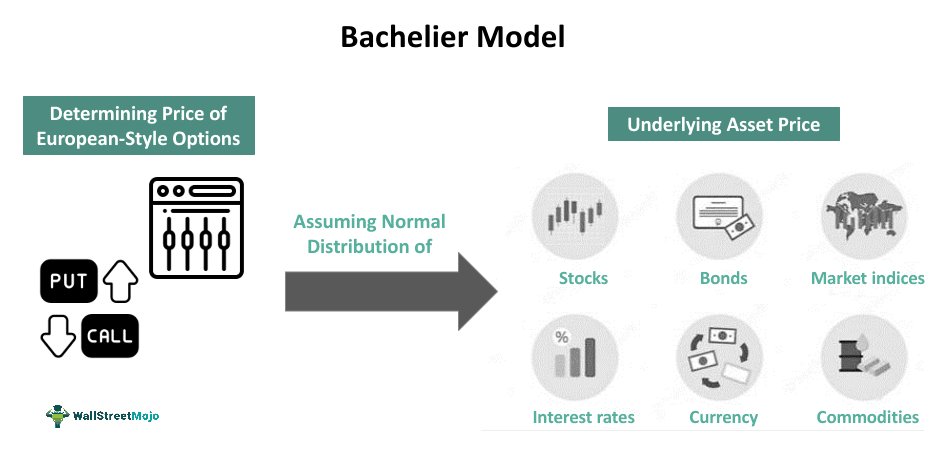
Louis Bachelier came up with the Brownian motion concept in the 1900s, which the Bachelier model employed to explore price dynamics. Later Fischer Black and Myron Scholes expanded the entire model in the 1970s. One utilizes this method for pricing options in markets where the underlying asset follows a normal or Gaussian distribution. This assumption implies that price changes follow a normal distribution and possess constant volatility.

What is Bachelier Model?

The Bachelier model is a mathematical framework that finds application in the pricing of European options on assets that do not pay dividends, assuming that the underlying asset follows a normal distribution.
It mostly finds use in modern quantitative finance for gauging the prices of less but constantly volatile short-term options, for instance - interest rate options or options on futures contracts.
The Bachelier model assumes constant price volatility throughout the option's lifespan based upon normal distribution, distinguishing it from the Black-Scholes model that assumes the options' price changes based on the log-normal distribution.

Bachelier Model Explained

The Bachelier model has been a revolutionary development in stochastic processes in modern quantitative finance. It aids in ascertaining the option price depending upon several factors, including the current price of the underlying asset, the option's strike price, the time to expiration, and the underlying asset's volatility. The model assumes Brownian motion that functions on the phenomenon that the underlying asset price is constantly variable, although such variation may be random and small.

The Brownian motion, which forms the basis of this mathematical model, was discovered by the great French mathematician Louis Bachelier in 1900 during his Ph.D. Thesis 'Théorie de la Spéculation.' He later came to be known as the Father of financial mathematics for his contribution to the world of speculation.

Hence, such a financial model is particularly valuable for pricing options on assets with relatively low volatility or short-term options. However, it may not be suitable for assets or options exhibiting significant skewness or kurtosis, as it assumes a symmetric normal distribution of price changes. It differs from the Black-Scholes model, which assumes that price changes adhere to a log-normal distribution.

While the Bachelier model is a well-established pricing framework, the Black-Scholes model is more widely adopted due to its ability to handle assets with log-normal distributed returns. However, the Black-Scholes was specifically designed for European-style options and may not accurately price other options or complex derivative securities.

Formula

In the Bachelier model, one computes the option price through the cumulative distribution function (CDF) of the standard normal distribution. The Bachelier option pricing formula for the European call or put option is as follows:

For Call Option Price: C=e-rT

For Put Option Price: P=e-rT

Where, d1=(F-K)T;
F represents the forward price;
K denotes the strike level or cap rate;
N(d1) signifies the CDF of the standard normal distribution evaluated at d1;
N(d1) signifies the CDF of the standard normal distribution evaluated at d1;
N(-d1) indicates the probability density function (PDF) of the standard normal distribution ascertained at d1;
σ represents the constant volatility of the underlying asset;
r denotes a risk-free discount rate;
T signifies the time to expiration of the option in years.

Examples

Check out these examples for a better idea:

Examples #1

Apart from the pricing of European call-and-put options, the Bachelier model is applicable to value interest rate options such as caps and floors. These options are derivatives that offer protection against fluctuations in interest rates. The Bachelier model assumes that the underlying interest rates conform to a normal distribution, facilitating the valuation of these interest rate options.

Example #2

Suppose the current price of an underlying asset for a European call option is $100 while its strike price is $110. Also, the time to expiration is one year, the risk-free interest rate is 0.05 (5%), and the underlying asset volatility is 0.2 (20%).

We can use the given Bachelier model formula for evaluating the call option price:

C=e-rT

Here, the e is the exponential function (approximately 2.71828).

To calculate the option price using a Bachelier model, we need to find out the value of d1 first.

d1=(F-K)T

d₁ = ($100 - $110)/0.2√1 = -$50

Also, calculate N(d1) and n(d1) using statistical tables or software, and find the values of N(d1) and n(d1) corresponding to the calculated d1 value, I.e., -$50.

Finally, evaluate the expression using the obtained values of N(d1) and n(d1) to calculate the price of the European call option using the above-mentioned Bachelier option pricing formula.

Please note that the Bachelier model assumes a normal distribution for the underlying asset's price and constant volatility. If the underlying asset follows a different distribution or the volatility is not constant, the Bachelier model may not be suitable, and alternative models, such as the Black-Scholes model, may be more appropriate.

Bachelier Model vs Black-Scholes

The Bachelier model and the Black-Scholes model are the financial frameworks that specifically find use in the pricing of European-style options. However, both these models differ from each other in the following ways:

Basis	Bachelier Model	Black-Scholes Model
Definition	It is a financial mathematics model used to determine the price of the European-style options that don't provide dividends based upon the assumption that the underlying asset price has a normal distribution and exhibits a Brownian movement.	It is a mathematical model that calculates the theoretical price of a call or put option while assuming that the markets are efficient. The underlying asset price change follows a geometric Brownian motion and a log-normal distribution.
Application	It is employed for gauging the price of those low-volatile European-style short-term options.	It is used for determining the theoretical price of European-style options, which can only be exercised at expiration.
Origin	It was discovered by the French mathematician Louis Bachelier in 1900. It is based upon Louis Bachelier theory of speculation.	It was developed by the economists; Fisher Black and Myron Scholes in 1973.
Popularity	Less commonly used or acknowledged framework	Renowned and widely recognized options pricing model
Assumptions	It is assumed that prices of the underlying asset are based upon Brownian motion, and returns are based upon normal distribution.	It is based on the following assumptions: 1. Returns are based upon log-normal distribution 2. Prices of the underlying asset are based upon Brownian motion, I.e., it constantly fluctuates 3. There are no dividend payouts made during the option's lifespan 4. Markets are efficient and frictionless with no transaction cost, and there are constant risk-free rates.
Formula	For Call Option Price: C=e-rTFor Put Option Price: P=e-rT	For Call Option Price: C(St,t)=N(d1)St-N(d2)PV(K)For Put Option Price: P(St,t)=N(-d2)Ke-r(T-t)-N(-d1)St
Limitations	Its application is limited to financial instruments that don't pay dividends. Also, it assumes constant volatility when it cannot be true in the real world.	The assumptions on which this model relies, such as risk-free returns and constant volatility throughout an option's lifespan, don't fit in the real-world scenario. Also, the belief in free-of-cost and continuous trading results in ignorance of brokerage charges and liquidity risk.

Frequently Asked Questions (FAQs)

1. What is the delta in the Bachelier model?

In the Bachelier model, the term "delta" refers to measuring an option price's sensitivity to small changes in the underlying asset's price. It quantifies the rate at which the option price changes relative to fluctuations in the underlying asset's price. It is the change in the price of the option to the change in the underlying asset price. Say, if the underlying price increases by $4 and the option price rises by $2, the delta is 0.5. Hence, it is a useful gauge for determining the hedge ratio.

2. What are the factors that affect an option's price?

The following factors influence the pricing of options:
- Underlying asset price
- Strike price
- Time to expiration
- Volatility
- Interest rate
- Dividends

3. Why is the Black-Scholes option pricing model so popular, although the Bachelier model has existed since 1900?

As the Black Scholes model assumes the log-normal distribution of the underlying assets, it is considered more reliable. It can further be used for various financial instruments like options with dividends, options on futures contracts and options on currencies.