Excel AVERAGEIF Function

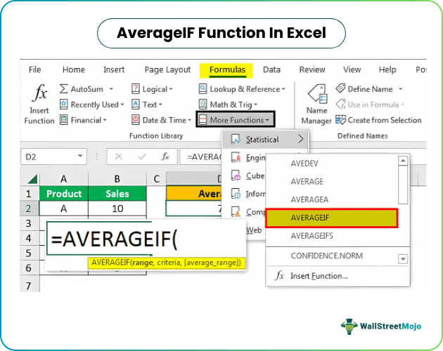
AverageIF in Excel calculates the average of the numbers just like the average function in Excel. But the only difference is that AverageIF is a conditional function, and it calculates the average only when the criteria given to the function are met. It takes three required arguments, a range followed by the criteria, and the average range.

For example, suppose we have a product dataset, and we need to know the product sales average. Using the Excel AVERAGEIF function, we can calculate the average of all the sales in a range of cells based on the specific criteria.

We have numerous Excel functions to work in different situations. For example, the AVERAGE function calculates the average of the range of cell values. Similarly, we can also calculate the average of specific values based on other columns. Based on the mentioned criteria, we can calculate the average of the numbers by using the AVERAGEIF function. In this article, we will take you through the function in excel, i.e., AVERAGEIF.

• The AVERAGEIF function is one of the Statistical functions in excel.
• It is used to calculate the average of the cells based on the criteria.
• The AVERAGEIF function was introduced in 2007.
• The syntax of AVERAGEIF function in excel is =AVERAGEIF(range,criteria,), where range denotes the range of cells with criterias; criteria denotes the cells for which the average has to be calculated.
• Both the range and criteria arguments of the AVERAGEIF function in excel are mandatory, and only the average_range argument is optional.

Let me explain to you the syntax of the AVERAGEIF function. It has three arguments to deal with. Below are the criteria.

• Range: The range of cells that has criteria values. In our above example, our range was “Product.”
• Criteria: From the Range for which item we need to take the average out, i.e., criteria. For example, in the above table, we need to take the average for which product out of all the products.
• : We need to select the number column we want to calculate the average.

The AVERAGEIF function calculates the average of specified numbers but is also based on supplied criteria.

For example, look at the below data sample.

We can easily tell the average sales from this data table by applying the AVERAGE function.

So, the average sale is 180 from the above data table. It is easy, but how do you tell what the average of the product “A” is?

That is where the AVERAGEIF function will help us. Here the criteria to calculate the average is Product “A.”

Let us learn how to use AVERAGEIF in Excel with detailed examples.

Example #1

Let us take the same data as an example.

So, the AVERAGEIF function calculates the average only for the Product “A” is 200.33, whereas the overall average is just 180.

Example #2

Now, look at the below data. Again, we have a product name, price, and the number of units sold in this data.

So, from the above list, we need to calculate the average unit sold when the unit price is >=25. So, we need to use the operator key greater than (>) in the criteria argument. Then, follow the below steps to calculate the average.

• Step 1: First, we must open the AVERAGEIF function in one of the cells.

• Step 2: Select range as the "Unit Price" column from B2 to B10.

• Step 3: Since we need to take the average only for the unit price >=25, we must enter the criteria as “>=25.”

• Step 4: The average range is the "Unit Sold" column from C2 to C10.

• Step 5: We are done with the formula. Close the bracket and press the "Enter" key to get the average unit sold number when the unit price is >=25.

So, when the unit price is >=25, average sales are 2,221 units. Similarly, now we will calculate the average sales when the unit price is <25.

So, when the price drops less than 25 per average sales of price is only 1,917.

Example #3

Wildcard characters are useful in excel functions. One of the problems with the AVERAGE or AVERAGEIF Excel function is it takes zero as one value and calculates the average value, including zero. Now for an example, look at the below data.

In the above image, the AVERAGE function calculates the average of the numbers from B2 to B6. So, we have five numbers from B2 to B6, but zero. So, we get the increased average when we calculate the average excluding zero.

So, we got an average of 7 now. But in this small data, we have easily identified the zero and applied the formula, but it is an arduous task in big data. So, we need to use the AVERAGEIF function to take the average of numbers other than zero.

For this case again, we need to use wild card characters. When the less than and greater than symbols are combined, it tells Excel not to count that so that the criteria will be “<>0.”

Like this, we can use the AVERAGEIF function to calculate the average based on some supplied criteria.

• All the empty cells are ignored by the formula for
• We will get #DIV/0! Error if the wrong criteria are supplied.
• Logical values "TRUE" and "FALSE" are treated as 1 and 0.
• We can use wildcard characters.

This article has been a guide to AVERAGEIF in Excel. We discuss calculating the average with the given criteria using an AVERAGEIF function, practical examples, and a downloadable Excel sheet. You can learn more about Excel functions from the following articles: -

• Excel Sumif Text
• AVERAGEIFS in Excel
• Combine SUMIF With VLOOKUP
• How to use COUNTIF Function in Excel?