Table Of Contents
What is AutoFill in Excel?
AutoFill in excel can fill a range in a specific direction by using the fill handle. The range is filled with values (numerical, textual or a mix) which are either copied from the initially selected cell or based on the pattern of the selected cells. The range can be filled downwards, upwards, rightwards or leftwards. A fill handle is a small square appearing at the bottom-right corner of a selected cell or range.
For example, type “abc” (without the double quotation marks) in cell E8. Select cell E8 and a fill handle appears at the bottom-right corner. Drag the fill handle in the following directions and the given output is displayed (without the double quotation marks):
- Downwards (till cell E12)–The text “abc” appears in the range E9:E12.
- Upwards (till cell E4)–The text “abc” appears in the range E4:E7.
- Rightwards (till cell I8)–The text “abc” appears in the range F8:I8.
- Leftwards (till cell A8)–The text “abc” appears in the range A8:D8.
Likewise, one can fill a range with a series of numbers. The number of the selected cell is copied in the different ranges, horizontally and vertically. It is also possible to fill the range with consecutive numbers (like 1-10).
A fill handle is an essential part of the AutoFill feature of Excel. On dragging or hovering the mouse over the fill handle, it changes from a square to a black plus sign. It must be noted that one can drag the fill handle in only one direction at one time. Moreover, the fill handle cannot be dragged diagonally.
Let us go through some examples to understand the working of the AutoFill feature in Excel.
#1–AutoFill Excel Options Explained
Example #1
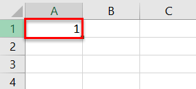
The following image shows a number in cell A1. We want to perform the following tasks:
- Copy the number of cell A1 to the range A2:A7 by using the AutoFill feature of Excel.
- Show and explain the different alternatives of the AutoFill options box.
The steps to perform the given tasks are listed as follows:
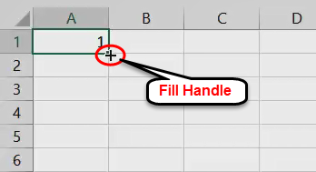
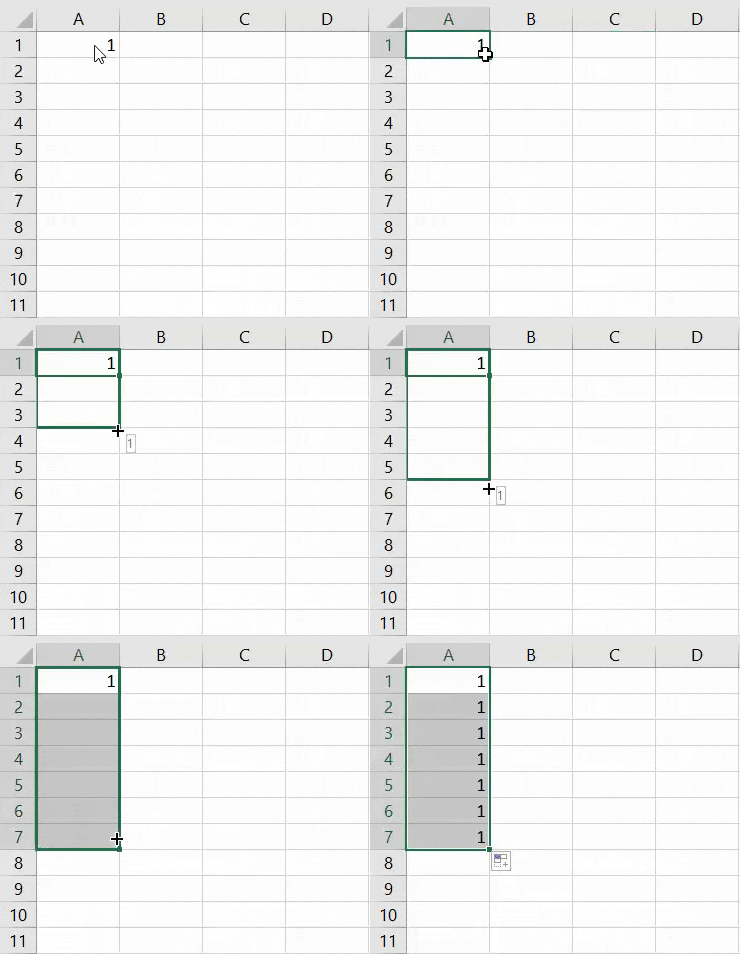
Step 1: Select cell A1. Hover the mouse over the lower-right corner of cell A1. A black plus sign appears, as shown in the following image. This plus sign (shown within the red circle) is the changed form of the fill handle, which appears as the cursor is placed on it.
Step 2: Drag the fill handle till cell A7. The range A2:A7 is filled with the number 1, as shown in the following image.
Hence, Excel has copied the value of the initially selected cell (cell A1) to a series of cells (A2:A7).
In the following pointers (step 2a to step 2g), the AutoFill options box is shown and its alternatives are explained.
Step 2a: The AutoFill options box is displayed immediately below the last cell, till which the fill handle is dragged (in step 2). The same is shown in the following image.
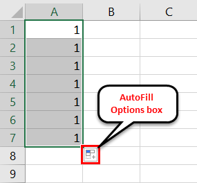
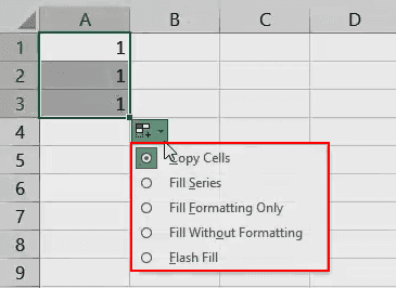
Step 2b: Click on the AutoFill options box. It displays various options. These options suggest the way the range (to which the fill handle is dragged) will be filled.
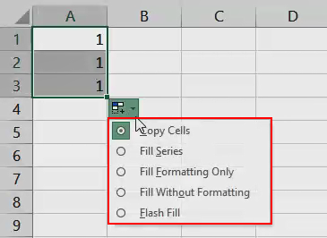
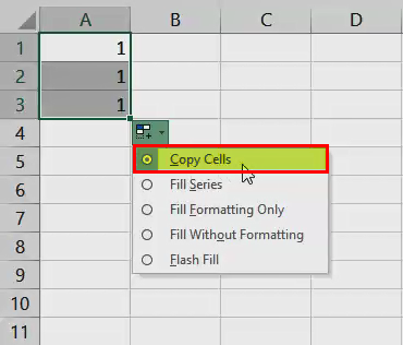
Step 2c: The first option is “copy cells,” as shown in the following image. This option copies the value of the initially selected cell to the entire selected range.
Step 2d: The second option is “fill series.” This option works with numerical values or a mix of numerical and textual values. It fills the range with a series of values based on the sequence detected. Excel identifies a sequence when more than one data cell is selected.
For instance, cells A1, A2, and A3 contain 1, 2, and 3. Select these cells and drag the fill handle downwards. The range is filled with a series of values incrementing by 1. This implies the following:
- Drag the fill handle downwards or rightwards and select the “fill series” option. It fills the range with an increasing order of numbers (like 4, 5, 6).
- Drag the fill handle upwards or leftwards and select the “fill series” option. It fills the range with a decreasing order of numbers (like 0, -1, -2).
Note: Remember that if Excel does not identify a sequence with the selection of two or more cells, one should select “fill series” from the AutoFill options box. With this selection, the default values that have been filled in the range are overwritten with sequential numbers.

Step 2e: The next option is “fill formatting only,” as shown in the following image. This option applies the formatting of the initially selected cell to the selected range. No values are entered in the selected range.
Note: The “fill formatting only” option is helpful in situations when formatting (of the initially selected cell) needs to be copied but values need to be entered manually.

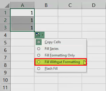
Step 2f: The fourth option is “fill without formatting,” as shown in the following image.
With this option, the value of the initially selected cell is copied to the selected range. If more than one cell is selected initially, this option fills the range based on a pattern. However, the formatting of the selected cell (or cells) is not copied.
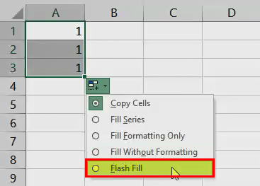
Step 2g: The fifth option is “flash fill.” This option fills the selected range automatically on the basis of the pattern detected. It is usually used to extract values from a data cell or combine the values of different data cells.
For instance, with flash fill, one can extract the middle name from the first, middle, and last name contained in a cell. Likewise, one can combine the first and last names contained in different cells.
For flash fill to work, one must enter the correct value (as desired) in the initial cell. As one begins typing the entry in the subsequent cell, Excel senses a pattern and fills the remaining range. Ensure that the output column (in which the desired value is entered) is adjacent to the source column.
Flash fill works for both numerical and textual values. It also works for a combination of numerical and textual values.
Note 1: The difference between “fill series” and “flash fill” is that the former identifies a sequence of numbers while the latter identifies a pattern of the selected values.
Note 2: The flash fill feature is available in Excel 2013 and the subsequent versions.
#2–AutoFill in Excel Using Two Starting Values
Example #2
The following image shows two numbers in cells A3 and A4. Use the AutoFill excel feature to fill the range A5:A14 in the sequence of the listed numbers.
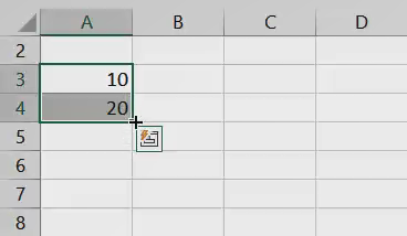
The steps to fill the range A5:A14 in the given sequence are stated as follows:
Step 1: Select cells A3 and A4.
Step 2: Drag the fill handle till cell A14, as shown in the following image. Excel senses a sequence and fills the range A5:A14 with numbers increasing by 10.
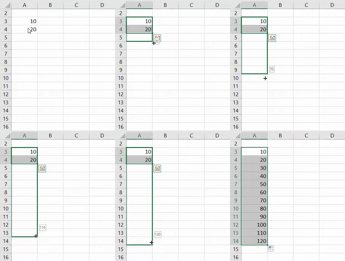
Likewise, if cells A3 and A4 contain 90 and 80 respectively, select them and drag the fill handle downwards. Excel fills the range A5:A14 with numbers decreasing by 10. In this way, the range can be filled in either increments or decrements of numbers.
Example #3
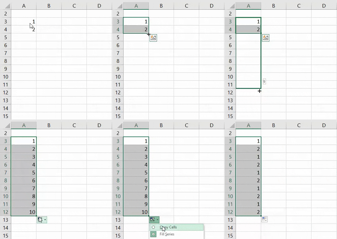
The following image shows two consecutive numbers in cells A3 and A4. Fill the range A5:A12 with the listed numbers appearing alternately.
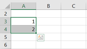
The steps to perform the given task are listed as follows:
Step 1: Select cells A3 and A4.
Step 2: Drag the fill handle till cell A12, as shown in the following image. Click the AutoFill options box and select “copy cells.”
Excel fills the range A5:A12 with numbers 1 and 2 appearing one after the other repeatedly.
#3–AutoFill Date and Time Values
Example #4
The following image shows a date in cell A4. Perform the following tasks:
- Fill the range A5:A12 with a series of dates by using the AutoFill feature of Excel. The difference between two consecutive dates should be equal to a day.
- Show and explain the additional alternatives (which were not covered in example #1) of the AutoFill options box.

The steps to perform the given tasks are listed as follows:
Step 1: Select cell A4. Drag the fill handle till cell A12. The same is shown in the following image.

Step 2: The output is shown in the following image. Excel fills the range A5:A12 with a series of dates. Each succeeding date is obtained by adding a day to the preceding date.
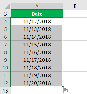
In the following pointers (step 2a to step 2e), the additional alternatives of the AutoFill options box have been showed and explained.
Step 2a: Click the AutoFill options box. The different options of this box are shown in the following image.

Step 2b: The “fill days” option (shown in the succeeding image) fills the selected range with a series of dates based on a pattern.
For instance, the cells A4 and A5 contain 11/12/2018 and 14/12/2018. Select these cells and drag the fill handle. Select “fill days” from the AutoFill excel options box. The range is filled with dates incrementing by 3 (like 17/12/2018, 20/12/2018, 23/12/2018).
Note: The “fill days” option observes the pattern in the days entered in the selected cells.

Step 2c: The “fill weekdays” option observes the pattern in days but fills the selected range with weekdays only. The weekends (Saturday and Sunday) are excluded from the series.
For instance, the cells A4 and A5 contain 10/12/2018 and 13/12/2018. Select these cells and drag the fill handle downwards. Select “fill weekdays” from the AutoFill excel options box. The series obtained are 17/12/2018, 20/12/2018, 24/12/2018, 27/12/2018, and so on. Hence, only the weekdays are returned as the output.

Step 2d: The “fill months” option (shown in the succeeding image) observes the pattern in the month entered in the selected cells.
For instance, enter 10/12/2018 and 13/12/2018 in cells A4 and A5. Select these cells and drag the fill handle. Select “fill months” from the AutoFill excel options box. The output is 10/1/2019, 13/1/2019, 10/2/2019, 13/2/2019, and so on.

Step 2e: The “fill years” option observes the pattern in the year entered in the selected cells. This option is shown in the succeeding image.
For instance, cells A4 and A5 contain 11/12/2018 and 12/12/2018 respectively. After selecting these cells and dragging the fill handle, select the “fill years” option. The series obtained are 11/12/2019, 12/12/2019, 11/12/2020, 12/12/2020, and so on.

Example #5
The following image shows a time value in cell A25. Fill the range A26:A34 with a series of time values incrementing by one hour. Use the “fill series” option of the AutoFill feature in excel.
Step 1: Select cell A25.
Step 2: Drag the fill handle till cell A34. Excel has filled the range A26:A34 with the different time values, as shown in the succeeding image.
Hence, the difference between two consecutive time values is one hour.

Step 3: Click the AutoFill options box. It shows that Excel has used the “fill series” option in this case. The same is shown in the following image.

#4–AutoFill Series Recognized by Excel
Example #6
In the following four images, one cell is filled with a value. We want to fill the range (immediately following the cell with value) downwards with a series of values. Use the AutoFill feature of Excel.
For simplicity, every image is preceded by an image number, title, and the steps to be performed.
Image 1–Days of a Week as the Series
- Select cell B3 which contains “Mon.”
- Drag the fill handle till cell B9.
Excel fills the range B4:B9 with the successive days of a week.
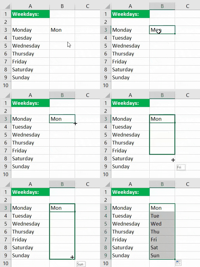
Image 2–Months in a Year as the Series
- Select cell B14 which contains “Jan.”
- Drag the fill handle till cell B20.
Excel fills the range B15:B20 with the successive months of a year.
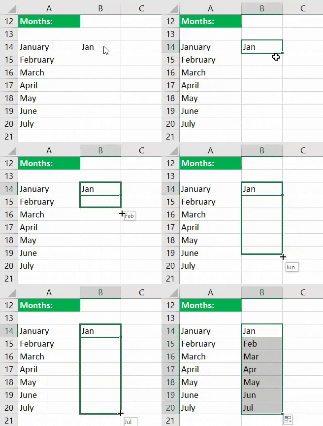
Image 3–Rank as the Series
- Select cell A25 which consists of “1st.”
- Drag the fill handle till cell A31.
Excel fills the range A26:A31 with the consecutive ranks.
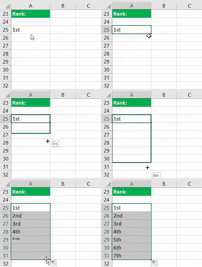
Image 4–Mix of Textual and Numerical Values as the Series
- Select cell A36 which consists of the string “week 1.”
- Drag the fill handle till cell A42.
Excel fills the range A37:A42 with the same text (week) but an increasing number (2 to 7).
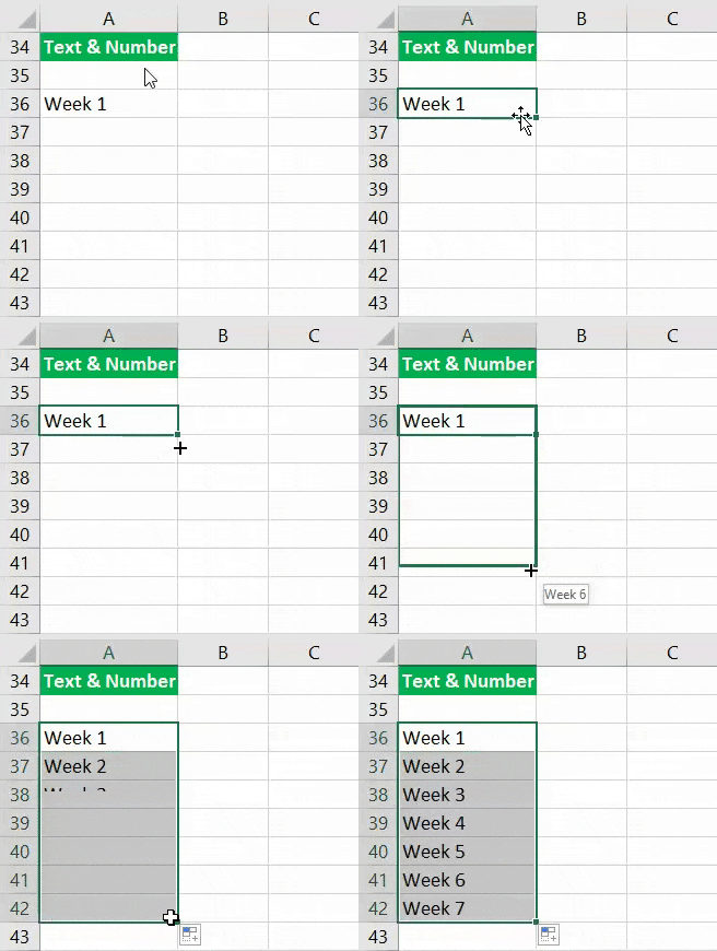
The four preceding images show the working of the “fill series” option of the AutoFill feature when only one cell is selected initially. However, one need not specifically select the “fill series” option as this is the default working of Excel in the given cases.
In other words, Excel recognizes certain values (entered in the initially selected cell) as a part of a series. Accordingly, it fills the selected range.
#5–AutoFill Values of Custom Lists in Excel
With a custom list, the different values (entries) of a series can be pre-defined in Excel. From these entries of the custom list, type one or more values in Excel. Excel fills the selected range with the entire series of the custom list.
Example #7
Create a custom list consisting of the names “Ian Smith,” “Patrick Henderson,” and “Samuel Samson.” Use the AutoFill feature of Excel to show the working of this list.
The steps to create a custom list in Excel are listed as follows:
Step 1: Go to the File tab.

Step 2: Click “options.”

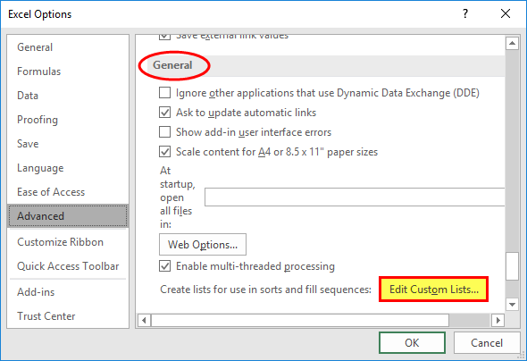
Step 3: The “Excel options” dialog box opens. From the pane on the left, click “advanced.” The same is shown in the following image.

Step 4: The “advanced options for working with Excel” are displayed on the right side. From the “general” section, click “edit custom lists.”
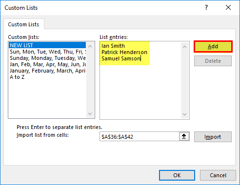
Step 5: The “custom lists” dialog box opens, as shown in the following image.
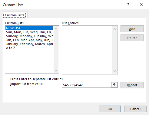
Step 6: Under “custom lists” (to the left), there are some lists defined by the system. The user-defined custom lists work the same way the system-defined lists work.
In the “custom lists” window, perform the following tasks:
a. Click “new list” under “custom lists.” Under “list entries,” type the names “Ian Smith,” “Patrick Henderson,” and “Samuel Samson.” These names are the different values (entries) of our custom list.
b. Press the “Enter” key after typing each entry (in “list entries”). Once all entries have been entered, click “add.”
c. Click “Ok” twice and exit from the “Excel options” dialog box.
The different list entries are shown in the following image.
Step 7: To check whether the user-defined custom list works or not, type the name “Ian Smith” in cell A1. Drag the fill handle till cell A11, as shown in the following image.
Note: One can enter any name of the user-created custom list. It need not necessarily be the first name of this list.
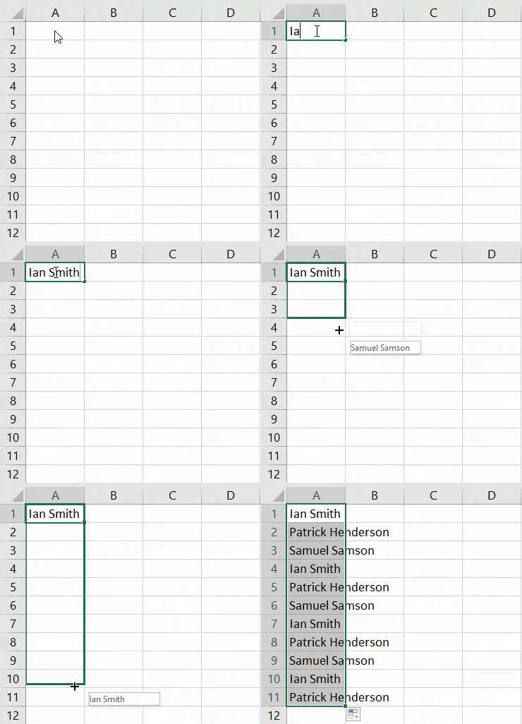
Step 8: The output is shown in the following image. Excel fills the range A2:A11 with the entries of the user-created custom list.
It must be noted that the sequence of the names in column A is the same as the “list entries” entered in step 6. Moreover, the names appear repeatedly in this column.

