AutoFilter In Excel

AutoFilter in Excel allows us to view specific rows while hiding the other rows. When Excel AutoFilter is added to the row's header, it gives us a drop-down menu in the header row.

AutoFilter in excel gives us multiple filter options, such as :

1. Equals to
2. Greater than
3. Less Than
4. Greater than or equal to
5. Begin with
6. Ends with
7. Contains
8. Does Not Contains

The first four are the number of filters, while the remaining are text filters.

There are two ways to use the AutoFilter in Excel:

1. In the "Data" tab, click on "Filter" under the "Sort & Filter” section.

2. Excel shortcut - Press Ctrl + Shift + L.

The options specify which rows of the Excel workbook are to be displayed.

Let us learn the use of Excel AutoFilters with a few examples:

AutoFilter in Excel - Example #1

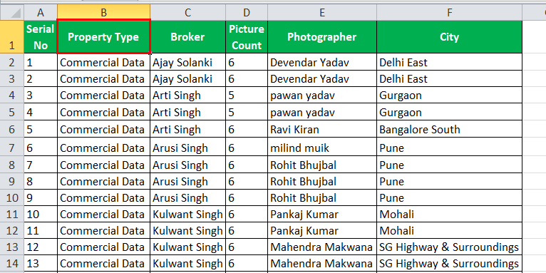
A real estate website has different property types of data, including residential and commercial. They have specific brokers and photographers who click the images for those real estate properties. The company also maintains the picture count in the properties taken by the photographer.

The task is to find which city has a picture count of 33, and broker Prateek has that property.

• Click on any row header that is on row 1.

• Click on “Filters” in the “Data” tab under the “Sort & Filter” section.

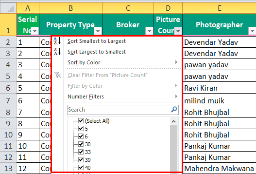
• The filter is applied in the row header, giving us a drop-down menu.

• Unselect all the counts by unchecking select all and select 33 for picture count.

• Select broker as "Prateek" by unchecking select all and selecting except "Prateek" in the "Broker" column.

• Our cities have 33 pictures, and broker "Prateek" has those properties.

By Excel AutoFilter, we have chipped our data. Therefore, the data which did not meet our criteria, i.e., picture count other than 33 or broker other than "Prateek," is hidden.

We have our desired data as we wanted.

AutoFilter in Excel - Example #2

Some students have scored marks in their annual exams in a teacher's class. For example, the teacher wants to know which student has scored above 50 in Maths and whose total is above 300.

• We will use a different approach to use filters this time.
• In the row header, press “Ctrl” + “Shift” + “L.”

• After the AutoFilter is applied, in the Maths column, uncheck select all and select values above 50.

• Now, select values above 200 by unchecking all and selecting values above 300.

• Now, we have those students who have scored above 50 in Maths, and the total is above 300.

AutoFilter in Excel - Example #3

In continuation with example 2, we can also use a custom filter.

But first, what is a “Custom Filter”?

A “Custom Filter” is an Excel filter option that allows us to put certain conditions to get our values. For example, in example 2, the condition marked above 50 in mathematics or above 300 in the total marks.

Let us learn custom filters by example 2.

• Select any cell in the row header.
• Press “Ctrl + Shift + L.”
• In the Maths filter, click on “Number Filters.” As the data is in numbers, a dialog box pops up.

• Our condition values are above 50, so select greater than, and another dialog box pops up.

Write 50 in the box where there is the text “is greater than.”

• Excel automatically filters the data in which the marks in Maths are above 50.

• Use the same approach and write “greater than 300” in the total column.

We have our result where the marks in mathematics are above 50, and the total is above 300.

1. Click on the row header to insert the filter.
2. The filter hides the data which does not meet the criteria.
3. We can remove the filter by any of the two options to use the filter and get the data back in the original format.

This article is a guide to AutoFilter in Excel. We discuss how to use AutoFilter Excel in Excel, along with Excel examples and downloadable Excel templates. You may also look at these useful Excel tools: -

• VBA AutoFilter
• Excel Add Filter
• Filter Shortcut in Excel
• Auto Format in Excel Tips
• Tally Chart in Excel