Table Of Contents

Array Formulas in Excel

Last Updated :

Blog Author :

Edited by :

Reviewed by :

Explanation of Array Formulas in Excel

Array formulas in Excel are powerful formulas that help us perform very complex calculations.

We learned from the above examples that these formulas in Excel simplify complex and lengthy calculations. There is one thing to remember. However, in example 2, we returned multiple values using these formulas in Excel. We cannot change or cut the cell's value as it is a part of an array.

Suppose we want to delete cell G6 Excel. It will give us an error. Even if we change the value in the cell type, any random value in the cell Excel will provide an error.

For example, type a number in cell G6 and press the “Enter” key. It may provide the following error,

Upon typing a random value 56 in cell G6, it may give an error that we cannot change a part of the array.

If we need to edit an array formula, go to the function bar and edit the provided values or range. If we want to delete the array formula, delete the whole array, i.e., cell range B6 to G6.

How to Use Array Formulas in Excel?

Let us learn an array formula by a few examples:

One can use array formulas in two types:

If we want to return a single value, use these formulas in a single cell, as in example 1.
If we want to return more than one value, use these formulas in Excel by selecting the range of cells as in example 2.
Press CTRL + Shift + Enter to make an array formula.

Example #1

A restaurant's sales data consists of each product's price and the number of products sold.

The owner wants to calculate the total sales done by those products.

The owner multiplies the number of items sold for each product then sums them up as in the given-below equation,

Also, he gets the total sales as given below:

But this is a lengthy task. If the data were bigger, it would be much more tedious. So instead, Excel offers array of formulas for such tasks.

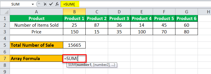
We will create our first array formula in cell B7.

The following are the steps to make the first array: -

In cell B7, type =SUM and press the “tab” button on the keyboard. It may open up the sum formula.
Select the cell range from B2 to G2.
Now, put an asterisk “*” sign after B2:G2 to multiply.
Select the cell range from B3 to G3.
Instead of pressing the “Enter” key, press “CTRL + SHIFT + ENTER.”

As a result, Excel may provide the total sales value by multiplying the number of products by the price in each column and summing them up. For example, in the highlighted section, we can see that Excel has created an array for cell range B2 to G2 and B3 to G3.

The above example explains how Excel array formulas return a single value for an array or set of data.

Example #2

With the same data, what if the owner wants to know the sales for each product separately, like sales of products 1 and 2?

He can either go a long way. In each cell, perform a function that will calculate the sales value.

The equation mentioned in cell B5 will be required to repeat for cells C4, D4, etc.

Again, it would be a tedious task if it were larger data.

In this example, we will learn how array formulas in Excel return multiple values for a set of arrays.

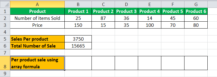
#1 - Select the cells where we want our subtotals, i.e., per product sales for each product. In this case, it is a cell range B8 to G8.

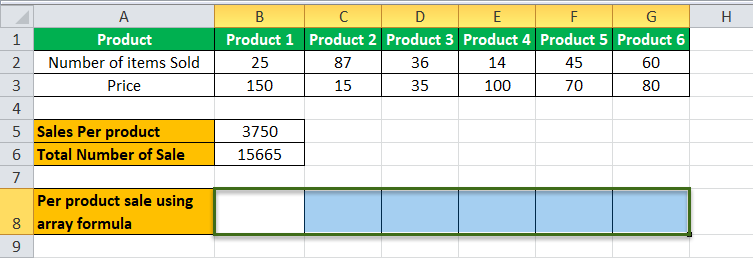
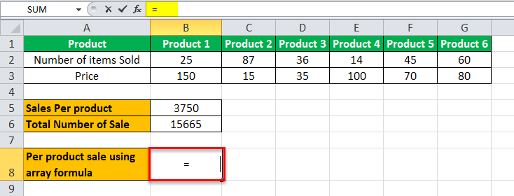
#2 - Type an equal to sign “=” a

#3 -Select cell range B2 to G2.

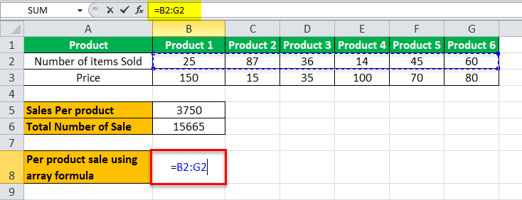
#4 - Type an asterisk “*” sign after B2:G2.

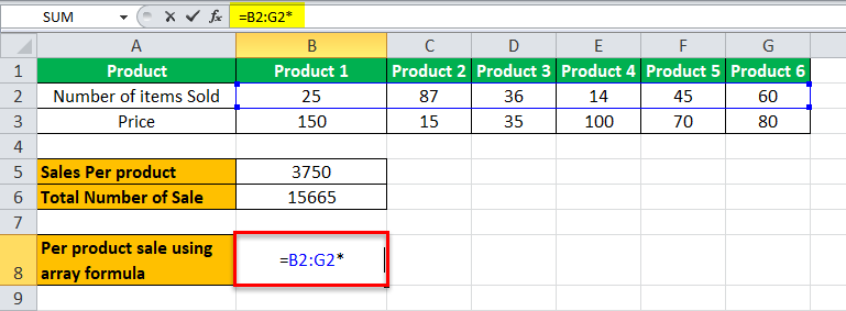
#5 - Now, select cell range B3 to G3.

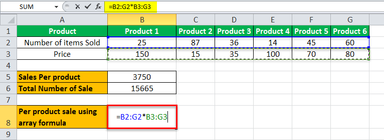
#6 - Do not press the "Enter" key for the array formula. Press “CTRL + SHIFT + ENTER” for array formula.

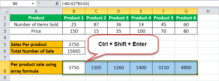
The above example explains how an array formula can return multiple values for an array in Excel.

Cells B6 to G6 are an array.

Example #3

For the same restaurant owner, he has the restaurant sales data for six months Jan, Feb, March, April, May, and June. He wants to know the average growth rate for sales.

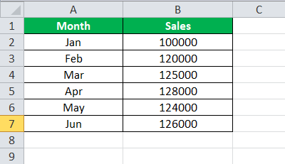
The owner can normally subtract the sales value of Feb month to Jan in cell C2 and then calculate the average.

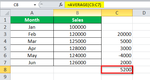
Again, it would be a tiresome task if this were larger data. So let us do this with the array in Excel formulas.

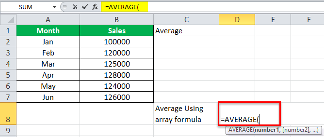
#1 – In cell D8, type =average. Then, press the "tab" button.

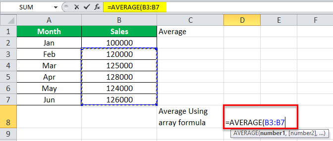
#2 – To calculate growth, we will need to subtract the values of one month from the previous month to select the cell range from B3 to B7.

#3 – Put a subtract (-) sign after B3:B7,

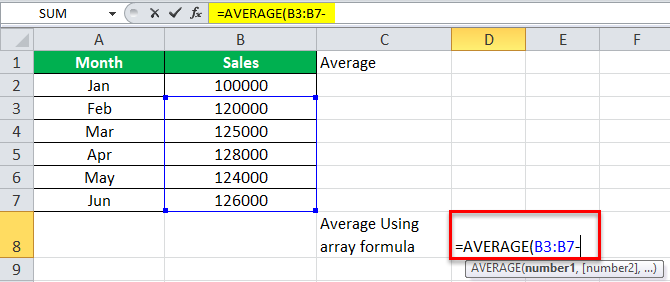
#4 – Now, select cells from B2 to B6.

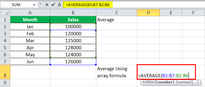
#5 – As for the array in Excel, do not press the "Enter" key. Press “CTRL + SHIFT + ENTER.”

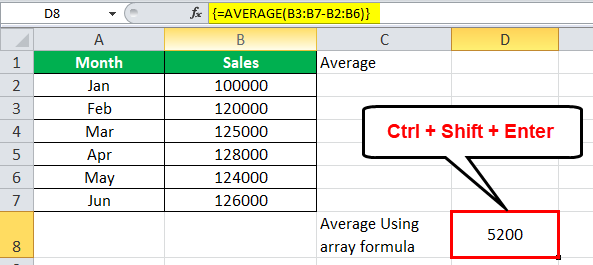
Array formulas in Excel easily calculated the average growth for the sales without any hassle.

The owner now does not require calculating each month's growth and performs the average function after that.

Things to Remember

These are also known as CSE Formulas or Control Shift Enter Excel Formulas.
Do not make parenthesis for an array; Excel itself does that. It would return an error or incorrect value.
Entering the parenthesis "{"manually, Excel will treat it as a text.
Do not press the "Enter" key. Instead, press "CTRL + SHIFT + Enter" to use an array formula.
We cannot change the cell of an array. So, to modify an array formula, either modify the formula from the function bar or delete the formula and redesign it in the desired format.