Table Of Contents
What Is Alphabetize In Excel?
Alphabetize in Excel is a method to sort a chosen data range or the entire sheet vertically or horizontally in alphabetical or reverse alphabetical order. We can use the Sort & Filter group options in the Data tab for alphabetizing data in Excel.
Users can utilize the alphabetizing options in Excel to automatically display a massive dataset in a specific order, which is a time-consuming process if sorted manually.
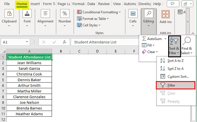
For example, the following dataset contains a student attendance name list.
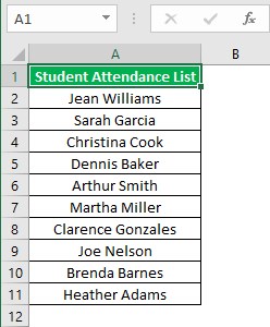
The requirement is to sort the names in ascending order.
Then, we can use the alphabetize in Excel ascending order option to achieve the required output.
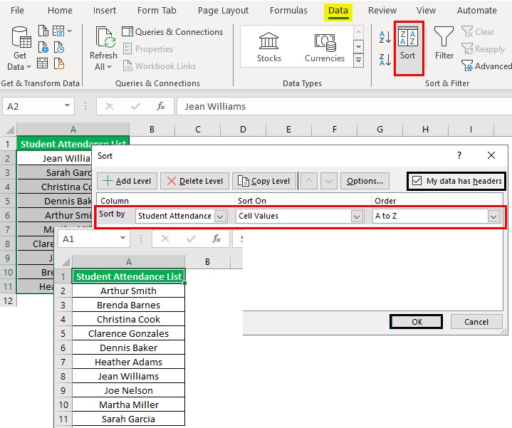
In the above alphabetize in Excel ascending order example, we choose the data range A2:A11 or cell A1 and select the Sort option in the Data tab.
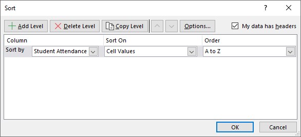
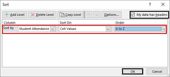
The Sort window will open. Since the dataset contains only one column, the Column Sort by field displays the existing column name. Also, the Sort On and Order fields show the default values, Cell Values and A to Z, which we will not change as they fit our requirements.
Finally, clicking OK in the Sort window shows the chosen range with the student names sorted in the required ascending order.
Table of contents
- Alphabetize in Excel is a technique to sort the given data in the alphabetical or reverse alphabetical order, row- or column-wise.
- Users can alphabetically sort data in Excel to make it more presentable quickly.
- We can use the Sort, Sort A to Z, Sort Z to A, and Filter options from the Data and Home tabs or use their keyboard shortcuts to sort data in a sheet alphabetically.
- We can sort Excel data alphabetically, keeping the rows together or by multiple columns, using formulas, and in individual rows and columns.
Shortcuts
The keyboard shortcuts to auto alphabetize in Excel are as follows:
- Press Alt + D + S, Alt + H + S + U, or Alt + A + SS, one after the other, to open the Sort window.
- Press Alt + H + S + S or Alt + A + SA, one after the other, to alphabetize the chosen data range in ascending order.
- Press Alt + H + S + O or Alt + A + SD, one after the other, to alphabetize the chosen data range in descending order.
- Press Ctrl + Shift + L simultaneously or Alt + A + T or Alt + H + S + F, one after the other, to apply the filter in the columns in the chosen range. Next, choose the first cell in the required column and simultaneously press the Alt + Down Arrow keys to open the specific column’s filter menu. After that, press the Down Arrow key once or S to choose the ascending or alphabetical sort option, Sort A to Z. Otherwise, press the Down Arrow key twice or O to choose the descending or reverse alphabetical sort option, Sort Z to A.
How To Use Alphabetize In Excel Using Sort & Filter?
We can auto alphabetize in Excel using the following Sort & Filter group options:
- Using Sort Option
- Using Filter Option
Method #1 – Using Sort Option
The first easy way to alphabetize in Excel using the Sort option is as follows:
- Select a cell in the range where we aim to alphabetize the data.
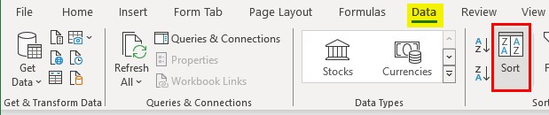
- Choose the Data tab - Sort option.
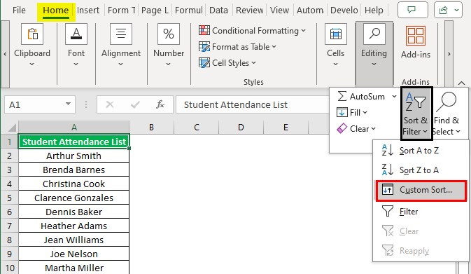
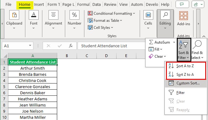
Alternatively, choose the Home tab - Sort & Filter option down arrow - The Custom Sort option.
The above step will open the Sort window.
- Ensure the My data has headers option is selected. Otherwise, the Sort option will include the column heading in the sorting process.
Next, click each field drop-down button to set their values according to the requirements.
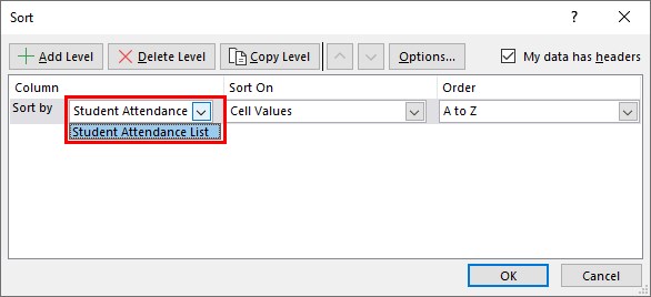
The first field, Column Sort by, is the column we aim to alphabetize or sort alphabetically.
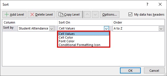
The second field, Sort On, helps us set the factor based on which we must sort data in Excel.
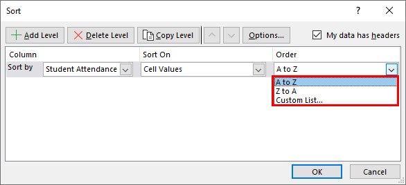
Next, the third field, Order, helps us select the sort order.
- Finally, click OK in the Sort window to close it and view the alphabetized data in the chosen range.
Furthermore, choose the required range and select the Data tab - The Sort A to Z or Sort Z to A option to alphabetize the chosen data in ascending or descending order quickly.
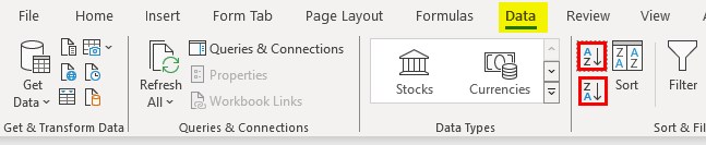
Alternatively, choose the required range and select the Home tab - The Sort A to Z or Sort Z to A option to quickly alphabetize the chosen data in ascending or descending order.
Method #2 – Using Filter Option
The second easy way to alphabetize in Excel using the Sort option is as follows:
- Select a cell in the range where we aim to alphabetize the data.
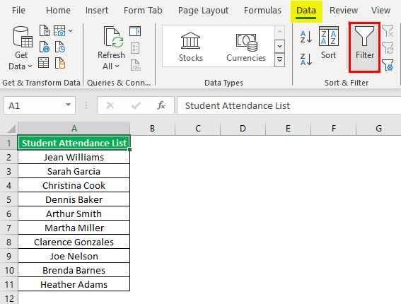
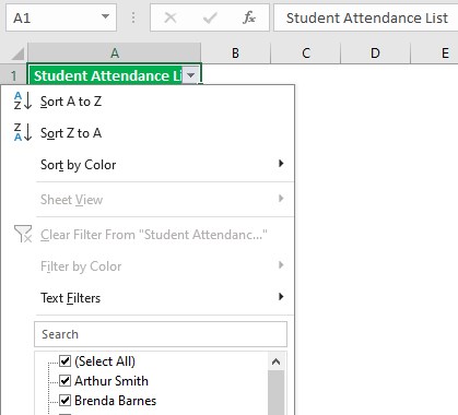
- Choose the Data tab - Filter option.
Alternatively, choose the Home tab - Sort & Filter option down arrow - The Filter option.
- The filter applies to the columns in the chosen range. We can click the filter drop-down button of the required column to open the filter menu. Next, choose the Sort A to Z or Sort Z to A option in the filter menu to alphabetize the data in ascending or descending order according to the requirements.
Examples
The following examples explain the alphabetizing methods in Excel to use them effectively.
Example #1 - Alphabetize In Excel Using Excel Formulas
We shall see how to alphabetize in Excel by last name.
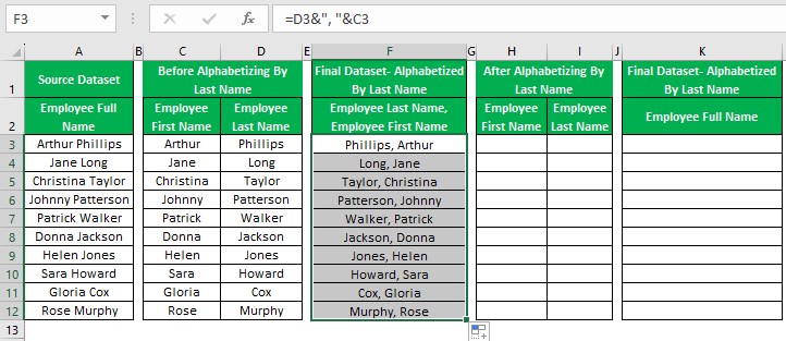
The following image shows a dataset containing employees’ full names in column A.
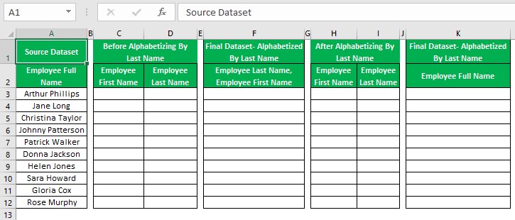
The aim is to sort the employees’ full names by their last name and display the output in column F.
Then, here is how to alphabetize in Excel by last name using formulas and the Sort option.
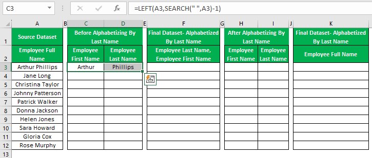
Step 1: Choose cell C3, enter the Excel LEFT function, and press Enter.
=LEFT(A3,SEARCH(" ",A3)-1)
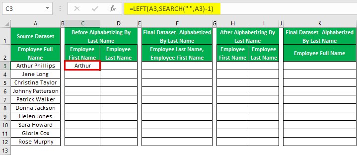
The SEARCH Excel function determines the position of the space character in the specified column A cell. Next, the formula deducts 1 from the position number the SEARCH() returns. After that, the LEFT() returns the number of characters specified as the second argument from the start of the value in the cell, supplied as the first argument.
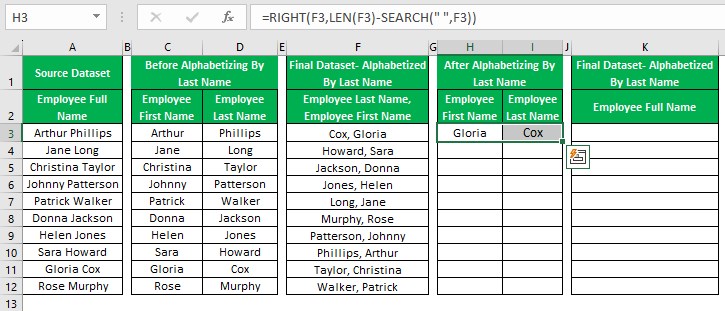
Next, choose cell D3, enter the Excel RIGHT function, and press Enter.
=RIGHT(A3,LEN(A3)-SEARCH(" ",A3,1))
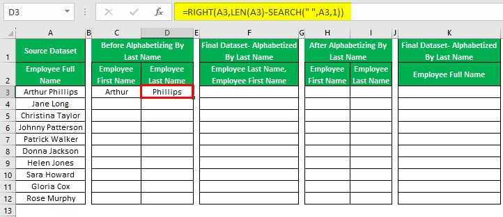
The LEN() returns the number of characters in the cited cell value. Next, the SEARCH() determines the Space character’s position or first occurrence. After that, the formula finds the difference between the Excel LEN function and SEARCH() outputs, a number supplied as the second argument to the RIGHT().
Next, the RIGHT() returns the number of characters (specified as the second argument) from the right end of the value in the cited cell.
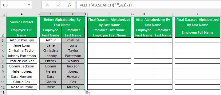
Step 2: Choose cells C3:D3.
Next, using the Excel fill handle, update the formulas in the column C and D cells in the range C4:D12.
Step 3: Choose cell F3, enter the following formula, and press Enter.
=D3&", "&C3
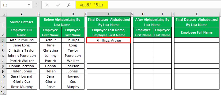
The formula concatenates the column C and D values, separated by a Comma and a space character.
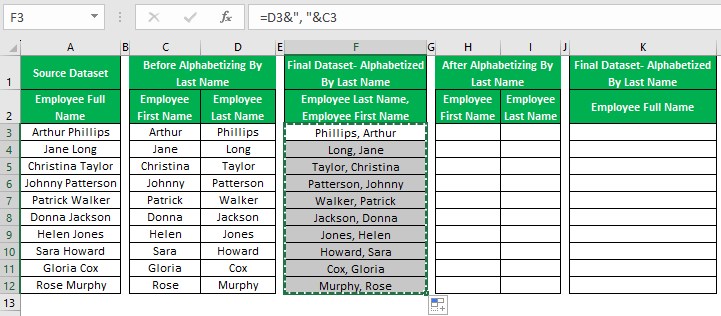
Next, using the fill handle, update the formulas in the remaining column F cells, F4:F12.
Step 4: Select the range F3:F12 and use Ctrl + C to copy the data in the chosen range.
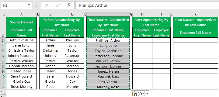
Step 5: Press Alt + E + S + V to open the Paste Special window and choose the Values option.
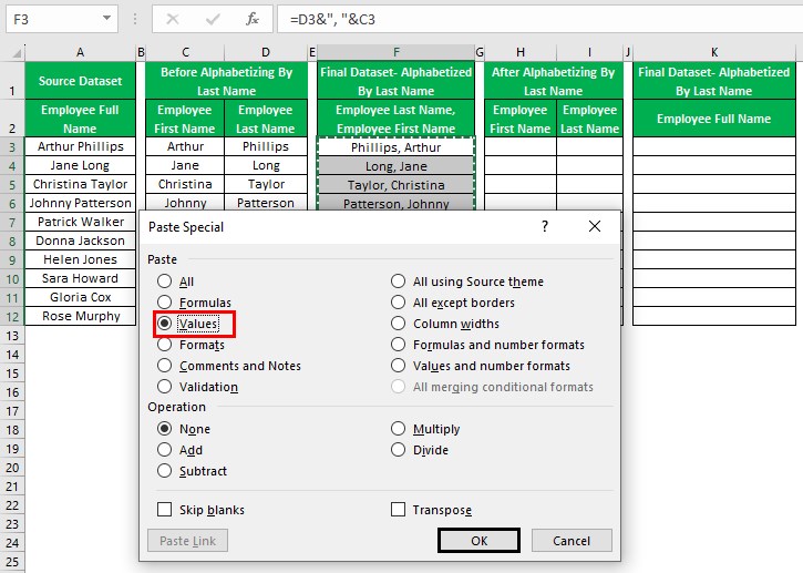
Next, clicking OK in the Paste Special window will close it, and the data in the range F3:F12 gets pasted as values, replacing the formulas.
Step 6: Select the range F3:F12 and choose Data - Sort.
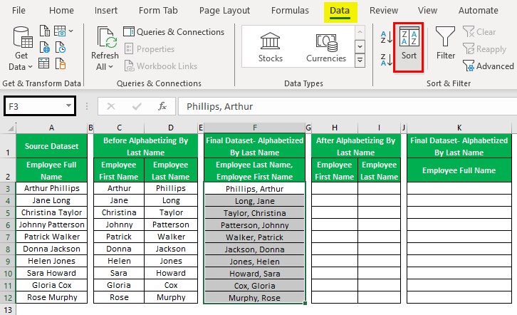
The Sort window will open, and the fields contain the values, indicating that the values are sorted by column F in ascending order.
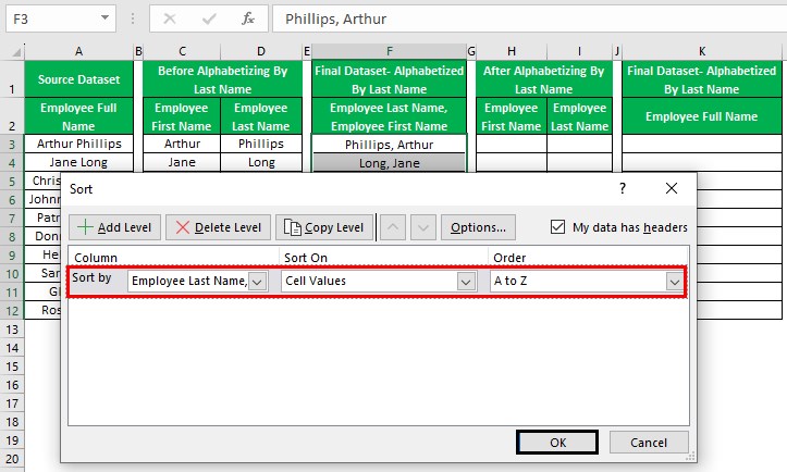
Clicking OK in the Sort window will close it, and the values in column F will appear sorted in ascending order based on the employees’ last names.

Furthermore, consider the task to display the full names alphabetized by the last name and in the same format as the source dataset (column A) in column K. Then, the steps are as follows:
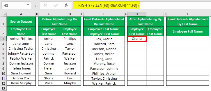
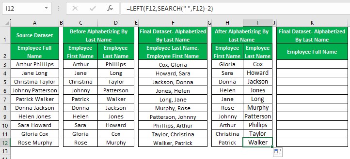
Step 7: Choose cell H3, enter the RIGHT(), and press Enter.
=RIGHT(F3,LEN(F3)-SEARCH(" ",F3))
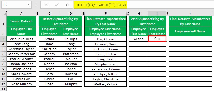
Next, choose cell I3, enter the LEFT(), and press Enter.
=LEFT(F3,SEARCH(" ",F3)-2)
Step 8: Choose cell H3:I3.
Next, using the fill handle, update the formula in the remaining columns H and I cells in the range H4:I12.
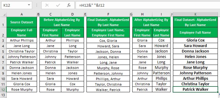
Step 9: Choose cell K3, enter the following formula, and press Enter.
=H3&" "&I3
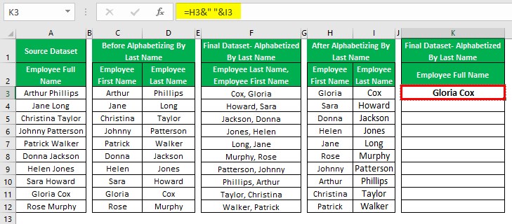
Next, using the fill handle, update the formula in the remaining target cells.
Example #2 - Alphabetize In Excel By Multiple Columns
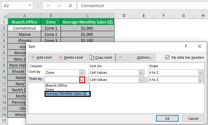
The following dataset contains a list of branch offices, their zones and average monthly sales figures.
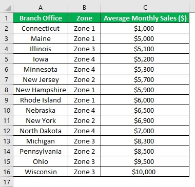
The task is to alphabetize the source dataset by zones in ascending order and then by the average monthly sales figures in descending order.
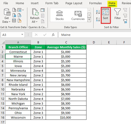
Step 1: Select a cell in the source dataset and choose Data - Sort.
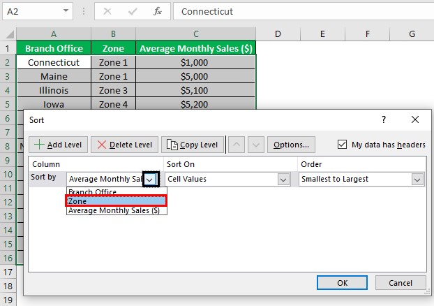
The Sort window will open, where we must set the Column Sort by field as Zone using its drop-down button and list. And since we must sort the cell values in ascending order, the remaining field values will be as depicted in the below image.
Step 2: Choose the Add Level option.
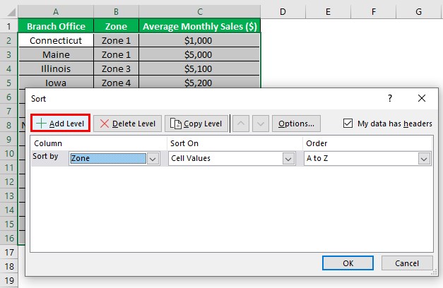
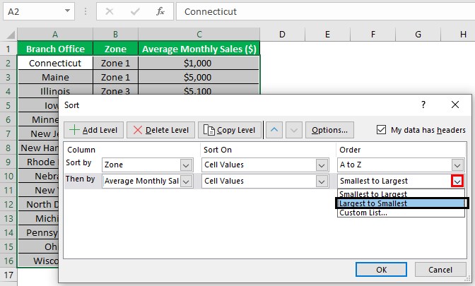
Excel shows another level to update the second sorting condition. We will set the Then by field as Average Monthly Sales ($).
Next, the Sort On field should be Cell Values and set the Order field value as Largest to Smallest using its drop-down button and list.
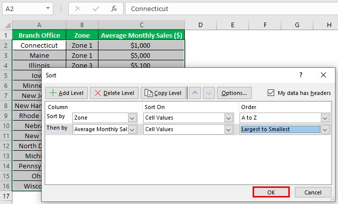
Finally, clicking OK in the Sort window will alphabetize the source dataset according to the specified conditions.
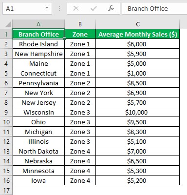
While the zones in column B appear sorted in ascending order, the average monthly sales values within each zone appear in descending order. Also, the corresponding column A values get rearranged according to the columns B and C sorted data.
Example #3 - Alphabetize In Excel By Keeping Rows Together
The following dataset contains a list of students and their Mathematics test scores.
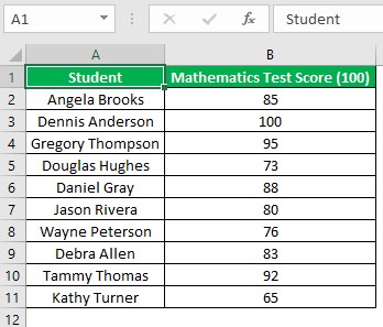
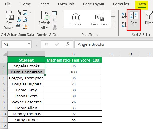
The aim is to alphabetize column A values, the students’ names, by keeping the rows together. Assume we choose multiple cells A2:A3 in the source dataset. Then, the steps are as follows:
Step 1: With the abovementioned cells chosen, select Data - Sort.
The Sort Warning window opens, showing two options. While the first option allows us to expand the selection, the second enables us to continue with the current selection.
Since we must include column B in the selection to alphabetize column A cells by keeping the rows, we shall choose the first option to expand the selection.
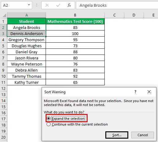
Next, select Sort in the Sort Warning window to proceed with the sorting process and open the Sort window.
Step 2: Set the Column Sort by field as Student using its drop-down button and list.
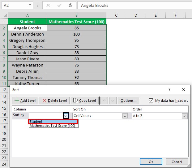
Next, set the Sort On and Order fields as Cell Values and A to Z, respectively.
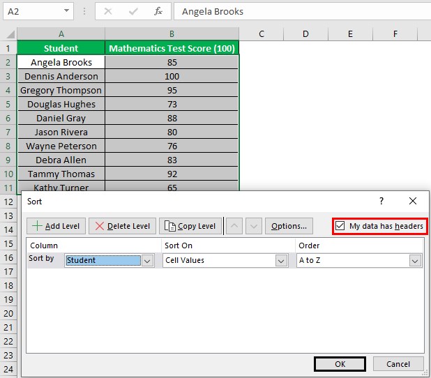
Finally, clicking OK in the Sort window will close it and display the source dataset alphabetized by keeping the rows intact.
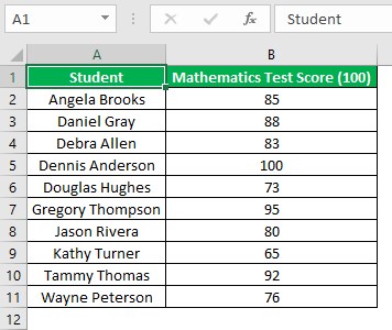
Thus, the students’ names appear sorted in ascending order, with their corresponding Mathematics test scores rearranged accordingly.
Example #4 - Put Rows In Alphabetical Order
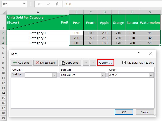
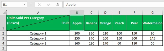
The following dataset shows fruits in row 1 and their units sold in different categories.
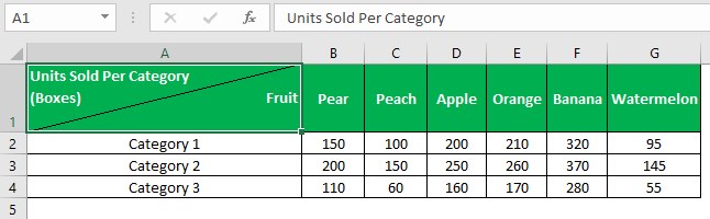
The aim is to alphabetically sort the fruits in row 1, leading to units sold data rearranged accordingly.
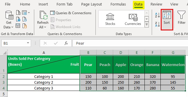
Step 1: Choose the range B1:G4 and select Data - Sort.
Step 2: The Sort window opens, where we must click the Options button.
Step 3: The Sort Options window will open, where we must choose the Sort left to right option.
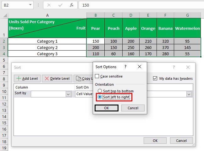
Clicking OK in the Sort Options window will change the Column Sort by field to Row Sort by field in the Sort window.
Next, since we must alphabetize the fruits in row 1, set the Row Sort by field as Row 1 using its drop-down button and list in the Sort window.
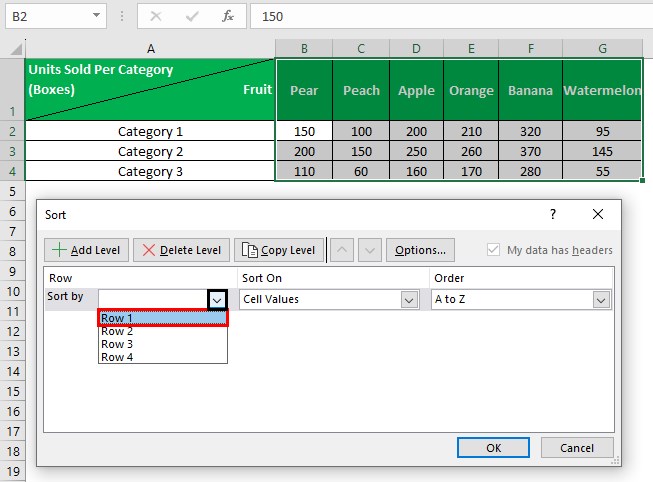
Next, we shall let the Sort On and Order fields contain the values Cell Values and A to Z.
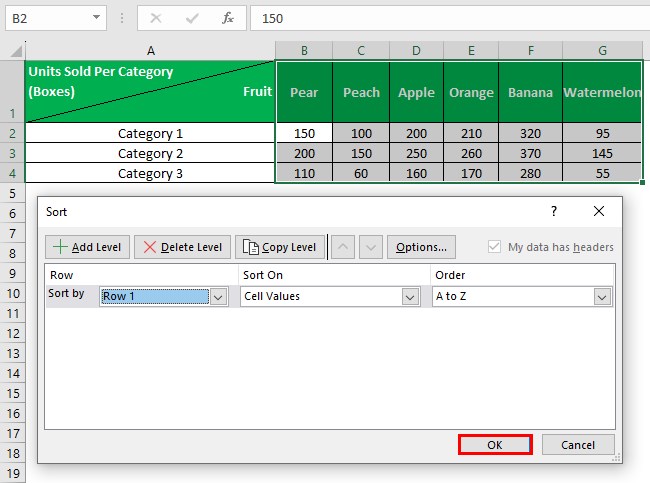
Finally, clicking OK in the Sort window will sort the fruits alphabetically, with the units sold data rearranged row-wise accordingly.
Problems
The issues with alphabetizing in Excel are as follows:
- Empty or hidden rows and columns can create problems while sorting alphabetically. In the case of a dataset containing blank rows or columns, the Sort option will sort the data until the first empty row or column. On the other hand, The Sort option ignores the data in the hidden rows and columns. So, the resulting dataset will not contain properly sorted data once we unhide the hidden rows and columns.
- If the column headings are unrecognizable, it can result in incorrect alphabetical sorting. When the column heading has the same format as the rest of the data in the column, the Sort A to Z and Sort Z to A options do not identify it as a column header. Instead, they consider the column heading as the data like the rest in that column and include it in the sorting process. It leads to the column heading appearing at another position in the sorted data based on the chosen sorting order. On the other hand, if we do not check the My data has headers checkbox in the Sort window, it will also cause the abovementioned issue.
Important Things To Note
- Ensure to choose one cell in the source dataset when using the Filter option to alphabetize in Excel.
- Ensure the source dataset does not contain blank and hidden rows and columns. Otherwise, the data will not get alphabetically sorted correctly.
- Ensure the column heading is recognizable and the My data has headers checkbox in the Sort window is selected to ensure the alphabetical sorting is correct.
Frequently Asked Questions (FAQs)
You can alphabetize each column individually in Excel using the following steps, explained with an example.
The following image shows the source dataset in the range A2:C5. It contains the list of members of three teams.
Here is how to sort each column in the source dataset individually and display the sorted data in the range A9:C11.
Step 1: Choose cell A9. Next, enter the INDEX() and press Ctrl + Shift + Enter to execute the expression as an array formula, as cited in the Formula Bar.
Next, choose cell B9, enter the INDEX(), and press Ctrl + Shift + Enter to implement the formula as an array formula.
Likewise, choose cell C9 and enter the INDEX() as an array formula.
Step 2: Select the range A9:C9.
Step 3: Using the fill handle, update the array formulas in the remaining target cells.
The COUNTIF() compares all the values in the same column with each other to return an array of their relative ranks. For instance, it returns {3;1;2} in column C, indicating Suzan is 3rd, Allen is 1st, and Harry is 2nd. So, we obtain the lookup array for the MATCH().
Next, the ROWS() provides the lookup value. Since we use the absolute and relative references, the returned number gets incremented by 1 as we move down a column. For instance, the lookup values for cells C9, C10, and C11 are 1, 2, and 3.
After that, the MATCH() searches for the lookup value, the ROWS() determined, in the lookup array, the COUNTIF() returned and gives its relative position. For instance, the lookup value for cell C11 is 3, which is in the 1st position in the lookup array, leading to the MATCH() returning 1.
Finally, the INDEX() determines the actual value based on its relative position in the column. In the case of cell C11, the function fetches the value in the range C3:C5, which is Suzan.
We can alphabetize in Excel on Mac using the following steps:
1. Choose a cell in the column we aim to sort.
2. Click the Data tab in the toolbar and locate the Sort option.
3. If the “A” appears on top of the “Z”, click that icon once. If the “Z” appears on top of the “A”, click the icon twice.
Please note that when the “A” is on top of the “Z”, the list will get sorted alphabetically. On the other hand, when the “Z” is on top of the “A”, the list will get sorted in reverse alphabetical order.
We can undo alphabetize in Excel using the following methods:
• Choose the Undo button from the Quick Access Toolbar or press Ctrl + Z.
• Use a helper column to obtain the original unsorted data.
Download Template
This article must be helpful to understand the Alphabetize In Excel, with its formula and examples. You can download the template here to use it instantly.
Recommended Articles
This has been a guide to What Is Alphabetize In Excel. We learn to alphabetize Excel data using sort & filter method and shortcuts, with Examples. You can learn more from the following articles –
