Table Of Contents

Address Function in Excel

Last Updated :

Blog Author :

Edited by :

Reviewed by :

Syntax of the ADDRESS Function

The syntax is stated as follows:

The function accepts the following mandatory arguments:

Row_Num: This is the row number used in the cell reference. The “row_num=1” represents row 1.
Column_Num: This is the column number used in the cell reference. The “column_num= 2” represents column B.

The function accepts the following optional arguments:

Abs_num (absolute number): This is the type of cell reference–absolute or relative. If this parameter is omitted, the default value is set at 1 (absolute). It can have any of the following values depending on the requirement:

Abs_num	Explanation
1	Absolute reference like “$A$1”
2	Relative column, absolute row like “A$1”
3	Absolute column, relative row like “$A1”
4	Relative reference like “A1”

A1: This is the reference style used. It can be either “A1” (1 or true) or “R1C1” (0 or false). If this parameter is omitted, the default style is “A1.”
Sheet_text: This is the name of the sheet used in the cell address. If this parameter is omitted, no worksheet name is used.

How to Use the Address Function in Excel? (With Example)

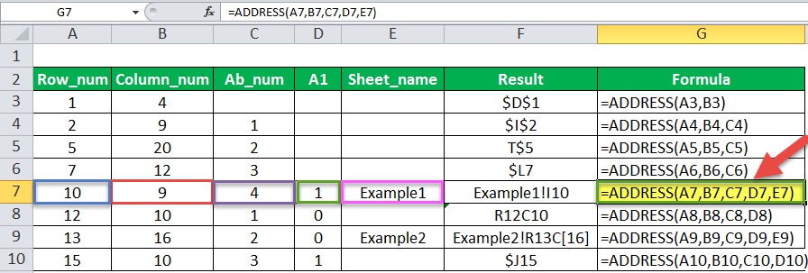
Let us consider the various possible outcomes of the ADDRESS function, as shown in the succeeding image.

The observations of a few rows are explained as follows:

1. The Third Row

The “row=1” and “column=4.”
The formula is “=ADDRESS(1,4).”
By default, the parameters “absolute number” and “reference type” are set at 1.
The result is an absolute address with an absolute row and an absolute column, i.e., “$D$1.”
The “$D” signifies the absolute column “4” and “$1” signifies the absolute row “1.”

2. The Fifth Row

The “row=5,” “column=20,” and “abs_num=2.”
The ADDRESS formula can be rewritten in a simpler form as “=ADDRESS(5,20,2).”
The reference style is set at 1 (true) when it has not been defined explicitly.
The result is “T$5,” which has an absolute row ($5) and a relative column (T).

3. The Seventh Row

We pass all the arguments of the ADDRESS function, including the optional ones.
The “row=10,” “column=9,” “abs_num=4,” “A1=1,” and “sheet_name=Example1.”
The address formula can be rewritten in a simpler form as “=ADDRESS(10,9,4,1,"Example1").”
The result is “Example1!I10.”
Since the “absolute number” parameter is set at 4, the result is a relative reference (“I10”).

How to Use the INDIRECT Function to Pass the Address?

The reference of a cell can be derived with the help of the ADDRESS function. However, if we are interested in obtaining the value stored in the Excel address of cells, we use the INDIRECT function. With this function, we can get the actual value through reference.

Syntax of the INDIRECT Function

Address function (Indirect function formula)

The function accepts the following arguments:

Ref_text: This is the cell reference supplied in the form of a text string.
A1: This is a logical value that specifies the style of reference. It can be either “A1” (true or omitted) or “R1C1” (false).

The first argument is mandatory, while the second is optional.

Let us consider an example.

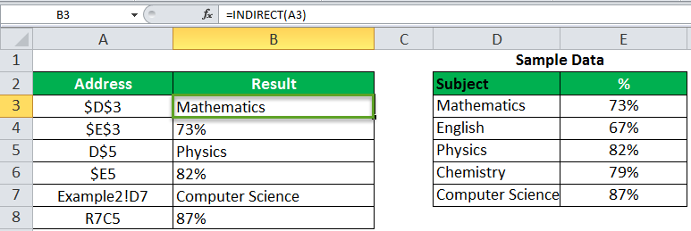
The data is given in the following image. We want to find the value of the cell reference passed in the INDIRECT function.

In the first observation, the “ADDRESS=$D$3.” We rewrite the function as “=INDIRECT(A3).”

In cell D3, under the sample data, the value is “Mathematics.” This is the same as the result of the INDIRECT function in cell B3.

Let us consider another example in which the reference style is R7C5.

Here, we must set the “ref_type” to “false” (0), so that the INDIRECT function can read the reference style.

The output of “=INDIRECT(A8,0)” is 87%.

Frequently Asked Questions

What are the uses of the ADDRESS function of Excel?

The uses of the function are listed as follows:
- It is used to address the first or the last cell in a range.
- It helps convert a column number to a letter and vice versa.
- It is used to construct a cell reference within a formula.
- It helps find the cell value from the row and column number.
- It returns the address of the cell with the highest value.

How does the ADDRESS function return the address of the cell with the highest value?

The ADDRESS function is used in combination with the MATCH function to return the cell address with the highest value. The formula is stated as follows:
“=ADDRESS(MATCH(MAX(B:B),B:B,0),COLUMN(B2))”
The MAX function returns the maximum value from the range “B:B.” The MATCH function looks for that maximum value and returns the row number (index). The column returns the column number of “B2.”

How does the ADDRESS function return the complete address of a named range?

The formula to return the full address of a named range is stated as follows:
“=ADDRESS(ROW(range), COLUMN(range)) & ":" & ADDRESS(ROW(range) + ROWS(range)-1, COLUMN(range) + COLUMNS(range)-1)”
“Range” is the named range whose address is required.
If the range address is required as a relative reference, the “abs_num” argument is set at 4. The formula can be rewritten as follows:
“=ADDRESS(ROW(range), COLUMN(range), 4) & ":" & ADDRESS(ROW(range) + ROWS(range)-1, COLUMN(range) + COLUMNS(range)-1, 4)”

The ADDRESS function creates a cell address from a given row and column number.
The syntax of the ADDRESS function is–“ADDRESS(row_num, column_num, , , ).”
The “row_num” and “column_num” are mandatory arguments, while “abs_num,” “A1,” and “sheet_text” are optional arguments.
The “abs_num” parameter can be set as follows:
- 1 or omitted–Absolute reference
- 2–Absolute row, relative column
- 3–Relative row, absolute column
- 4–Relative reference
The reference style can be set at either “A1” (1 or true) or “R1C1” (0 or false).
The default reference style is “A1.”
The INDIRECT function helps obtain the value stored in the Excel address of cells. The syntax of the INDIRECT function is–“INDIRECT(ref_text, ).”