Filter in Excel

Last Updated :

Blog Author :

Edited by :

Reviewed by :

Table Of Contents

What is Filter in Excel?

The filter in excel helps display relevant data by eliminating the irrelevant entries temporarily from the view. The data is filtered as per the given criteria. The purpose of filtering is to focus on the crucial areas of a dataset. For example, the city-wise sales data of an organization can be filtered by the location. Hence, the user can view the sales of selected cities at a given time.

A filter is necessarily required when working with a huge database. Being a widely used tool, the filter converts a comprehensive view into an easy-to-understand one. To apply filters, the dataset must contain a header row which specifies the name of every column.

What is Filter in Excel?

How to Filter in Excel?

It is good to work with filters because they fit our needs the way we want to. In order to filter data, select the entries to be visible and deselect the rest of the items.

The three methods to add filters in excel are listed as follows:

With filter option under the Home tab
With filter option under the Data tab
With the shortcut key

Let us consider a dataset to go through the three methods of adding filters.

The following table shows the invoices issued to the buyers of different cities. We want to filter the data using different methods.

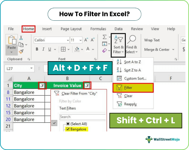
In the Home tab, there is a “filter” option under the “sort and filter” drop-down of the “editing” section, as shown in the following image.

Step 1: Select the data and click “filter” under the “sort and filter” drop-down.

Step 2: The filters are added to the selected data range. The drop-down arrows, shown within the red boxes in the following image, are filters.

Step 3: Click the drop-down arrow of the column “city” to view the different names of the cities.

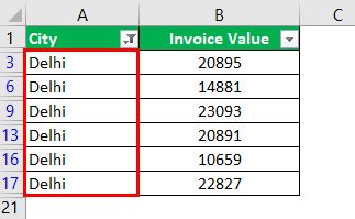
Step 4: To see the invoice values of “Delhi” only, select “Delhi” and uncheck all the remaining boxes.

Step 5: The data for the city “Delhi” is filtered and displayed in the following image.

In the Data tab, there is a “filter” option under the “sort and filter” section, as shown in the following image.

Method 3: With the Shortcut key

The keyboard shortcuts are a good way to speed up the daily tasks. Select the data and add the filter using either of the following shortcuts:

Press the keys “Shift+Ctrl+L” together.

Press the keys “Alt+D+F+F” together.

Note: The preceding shortcuts for adding filters are toggle keys. Repetitive pressing helps to turn on and turn off the filters.

How to Add Filters in Excel?

We can filter numbers using advanced techniques. Let us consider some examples to understand the working of filters in Excel.

Example #1–“Number Filters” Option

Working on the data under the preceding heading (methods of filtering in Excel), we want to apply the following filters:

a. To filter column B (invoice value) for numbers greater than 10000

b. To filter column B for numbers greater than 10000 but less than 20000

Let us go through the two cases one by one.

a. Filter numbers greater than 10000

Step 1: Open the filter in column B (invoice value) by clicking on the filter symbol.

Step 2: In “number filters,” choose the “greater than” option, as shown in the following image.

Step 3: The “custom autofilter” box appears.

Step 4: Enter the number 10000 in the box to the right of “is greater than.”

Step 5: The output displays the invoice values greater than 10000. The symbol within the red box is the filter icon. It indicates that the filter has been applied to column B.

b. Filter numbers greater than 10000 but less than 20000

Step 1: In “number filters,” choose the “greater than” option.

Step 2: In the “custom autofilter” box, select “is less than” in the second box to the left-hand side. This is shown in the following image.

Step 3: Enter the number 10000 in the box to the right of “is greater than.” Enter the number 20000 in the box to the right of “is less than.”

Step 4: The output displays the invoice values greater than 10000 but less than 20000.

Working on the data under the preceding heading (methods of filtering in Excel), we have replaced the first column (city) with product IDs.

We want to filter the details of product ID “prd 1.”

The steps are listed as follows:

Step 1: Add filters to the columns “product ID” and “invoice value.”

Step 2: In the search box, enter the value that is to be filtered. So, enter “prd 1.”

Step 3: The output displays only the filtered value from the list, as shown in the following image. Hence, we can see the invoice value of the product ID “prd 1.”

Option while you Drop Down the Filter Function

Sort A to Z and Sort Z to A: If you wish to arrange your data ascending or descending order.
Sort by Color: If you want to filter the data by color if a cell is filled by color.
Text filter: When you want to filter a column with some exact text or number.
Filter cells that begin with or end with an exact character or the text
Filter cells that contain or do not contain a given character or word anywhere in the text.
Filter cells that are exactly equal or not equal to a detailed character.

For example:

Suppose you want to use the filter for a specific item. Click on to text filter and choose equals.

It enables you the one dialogue, which includes a Custom Auto-Filter dialogue box.

Enter fruits under category and click Ok.

Now you will get the data of fruits category only as shown below.

The Techniques of Filtering in Excel

The following techniques must be followed while filtering data:

If the dataset is large, type the value to be filtered. This filters all the possible matches.
If numerical data has to be filtered by specifying the greater than or the less than number, use the “number filters” option.
If data has to be filtered by the color of specific rows, use the “filter by color” option.

Frequently Asked Questions

1. What are filters and how to add them in Excel?

Filtering is a technique which displays the required information and removes the unwanted data from the view. It helps the user focus on the relevant data at a given time.

The steps to add filters in Excel are listed as follows:
• Ensure that a header row appears on top of the data, specifying the column labels.
• Select the data on which filters are to be added.
• Add filters by any of the three given methods.
o Click the “filter” option under the “sort and filter” (editing section) drop-down of the Home tab.
o Click the “filter” option under the “sort and filter” section of the Data tab.
o Press the keys “Shift+Ctrl+L” or “Alt+D+F+F.”

Note: As soon as the filters are added, a drop-down arrow appears on the particular column header.

2. How to apply filters to one or more columns?

The steps to apply filters to one or more columns are listed as follows:
• Click the drop-down arrow of the column to be filtered.
• Uncheck the “select all” option which helps deselect all data.
• Select the boxes to be displayed.
• Click “Ok.”
The drop-down arrow changes to the filter icon as soon as a filter is applied. When filters are applied to multiple columns, the filter icon appears on each one of them. Hovering over the filter icon shows the filters that have been applied.

Note: The drop-down arrow on a column header indicates a filter is added. The filter icon indicates a filter has been applied.

3. How to use filters in Excel?

The filters can be applied to numbers, text values, and dates. These cases are discussed as follows:
Filter numbers
• Click on the “number filters.”
• Select any of the options like “equals,” “does not equals,” “greater than,” “less than,” “between,” “above average,” and so on.
• Specify the required fields in the dialog box that appears. This box may or may not be displayed.

For instance, in “equals,” enter the number against which the values should be compared. The filtered results show the matching numerical values.

Filter text and date values
• To filter text and date values, select “text filters” and “date filters” from the respective drop-down arrows.
• The “text filters” allow filtering text strings which contain specific characters or words. The “date filters” allow filtering dates for a particular year, month, week, and so on.

Note: The “plus” and the “minus” sign of the date filters are used for expanding and collapsing the various levels respectively.