3-D Reference in Excel

Last Updated :

21 Aug, 2024

Blog Author :

Edited by :

Reviewed by :

Table Of Contents

What is a 3-D Cell Reference in Excel?

As the name suggests, a 3-D reference means a three-dimensional reference. It means referring to something specific apart from the normal view. It is a powerful referencing, performed when we have multiple data in various worksheets with some common data in all the sheets. It will be a tedious task if we have to make calculations based on referencing each sheet manually. Instead, we can use the 3-D reference, which will refer to all the sheets at once in Excel workbook.

For example, suppose you must add or consolidate the budget data from various organizations or departments. You may use a 3-D reference. It is a valuable and convenient approach to several worksheets that can adopt the same pattern and cells on each worksheet consisting of the same data type. It can also help you add another worksheet and move it into the range where your formula is applied.

What is 3D Cell Reference in Excel?

Explanation

It means referring to some data to any other address in the digital world.

In Excel, 3-D cell referencing means referring data to other worksheets, making calculations, or building reports in another worksheet. It is one of the exceptional features of Excel.
It refers to a specific cell or range of cells in many worksheets. For example, we have a product price list in a different worksheet and the product count sold in another. We can calculate the product's total sales by referencing the data in the other worksheets.

How to Use 3-D Cell Reference in Excel? (With Examples)

Example #1

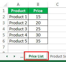
Let us begin with the example of the product explained. First, we have the price list of some products in sheet one, named the "Price List."

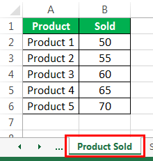
And we have an amount of product sold in worksheet 2, renamed "Product Sold."

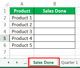
Now, we will calculate the product sales in sheet 3, renamed “Sales Done.”

In cell B2, type the formula "=" and refer to sheet 1-a price list. Then, select the price for the first product, product 1.

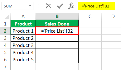
We can see that Excel's function bar references the first price list sheet to the B2 cell.

Now, put an asterisk sign for multiplication in Excel.

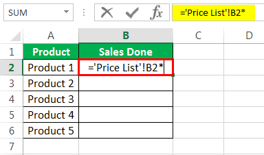
Now refer to Sheet 2, a product sold. Next, select the count of the product sold, cell B2.

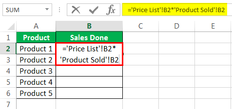
We can see that Excel's function bar references the second sheet of the product sold to cell B2.

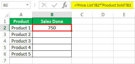
Press the “Enter” key. As a result, we have the sales done by-product 1.

Now, drag the formula to cell B2. Excel automatically calculates the sales done by the other products by reference to their respective price list and the count of products sold.

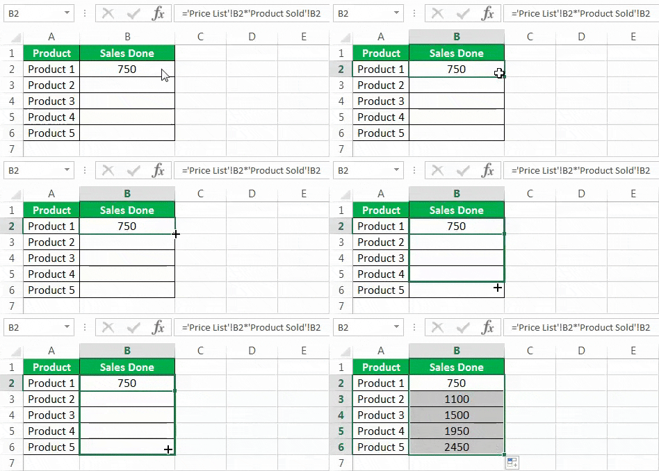
In the above example, we gave references from two sheets, which are Sheet 1 (Price List) and Sheet 2 (Product Sold), and calculated the sales done in the third worksheet (Sales Done).

It is called 3-D cell reference in Excel.

Example #2

Suppose we have a student's quarterly and half-yearly marks for five subjects, and the total marks need to be calculated in another worksheet.

One workbook is for quarter 1, and the data is for quarter 1.

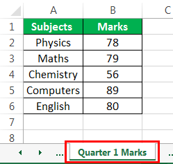
Similarly, we have marks for half-yearly and quarter 2.

Data for Half Yearly.

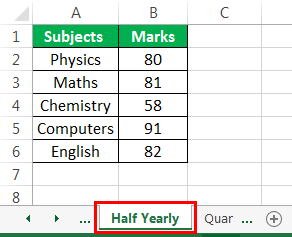
Data for Quarter 2.

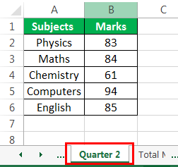
Now, we will calculate the total marks in another workbook by 3-D referencing.

In the Total Marks worksheet type,

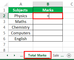
Start referring to the marks of different quarters and a half-yearly.

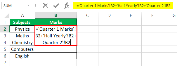
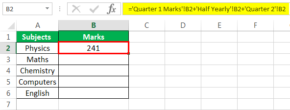
Press the "Enter" key. Hence, we obtained the total marks for the first subject.

Now, drag the formula to the last subject. As a result, we will have marks for all the subjects.

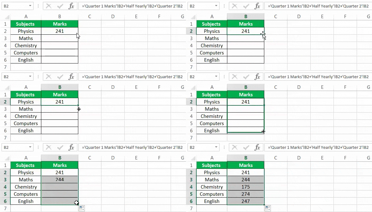
We have calculated the total marks for all five subjects by 3-D reference.

Example #3 – Creating a Chart with 3-D Reference

We cannot only make calculations but also can create charts and tables through 3-D reference. In this example, we will learn to make a simple chart using a 3-D cell reference in Excel.

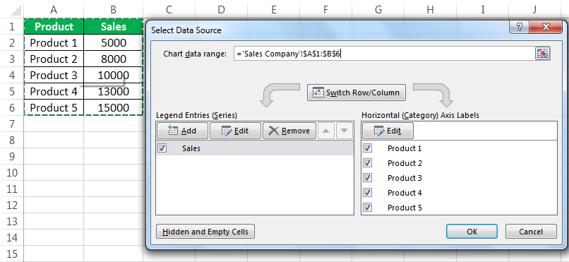
Let us consider that we have sales data for a company in a worksheet. Below is the data:

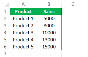
We will make a chart in another worksheet using the same data above.

In another worksheet, select any chart for this example. For example, I have chosen 2-D Column Chart.

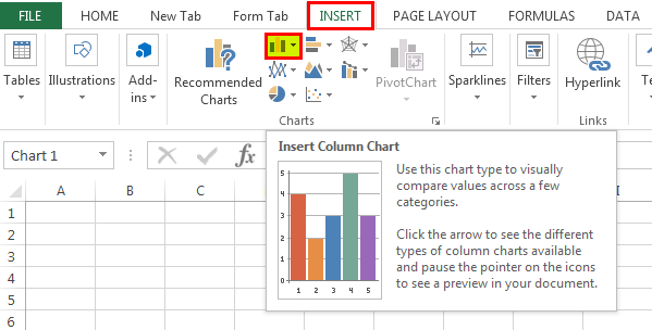
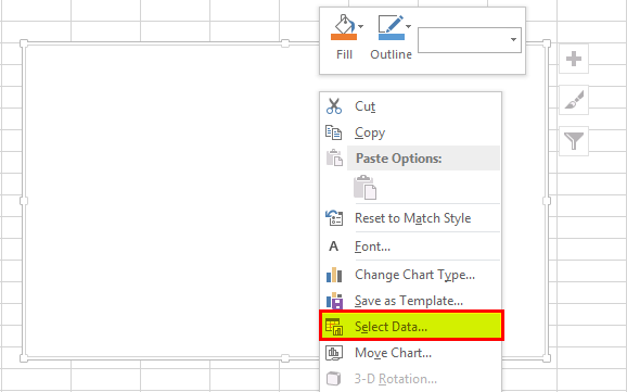
A blank chart appears. Now, right-click on it and click on "Select Data."

A dialog box opens up. In the chart data range, select the data in the other worksheet, which is the company sales data.

Our selected chart is created in the other worksheet by clicking "OK."

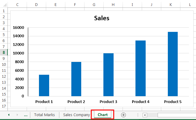
We have successfully made a chart using a 3-D reference.

Explanation of 3-D Cell Reference in Excel

A 3-D reference refers to different tabs or worksheets in the same workbook. Therefore, the data must be in the same pattern if we are required to manipulate the workbook data.

Suppose we have data in a workbook in the C2 cell and use a 3-D reference to calculate the value in another sheet in the D2 cell. If the data is moved from the first C2 cell by any chance, then Excel can still refer to the same C2 cell as earlier, whether it is a null value or any other value.

As explained earlier, 3-D referencing means referring data to other worksheets and making calculations or building reports in another worksheet. It relates to many cells in different worksheets, given that they are in the same pattern.

Things to Remember

The data must be in the same pattern in all the worksheets.
Excel can still refer to the specific cell range if the worksheet is moved or deleted.
Any worksheet added between the referencing worksheet will also alter the result because Excel can still refer to the specific cell range.